Lesson 1-1: Finite Difference Formula and Forward Difference

Before delving into numerical derivatives, let's review the mathematical definition of a derivative. The derivative of a function \(f(x)\) is defined as \[f'(x) = \lim_{{h\rightarrow 0}} \frac{f(x+h) - f(x)}{h}.\]

Building upon this formula, consider the following approximation of the derivative \(f'(x)\) of the function \(f(x)\) using a sufficiently small \(h\). \[ f'(x) \approx \frac{f(x+h) - f(x)}{h}. \tag{1}\] This approximation to the derivative using a finite width \(h\) is known as the finite difference approximation. Specifically, the expression in Eq. (1) is termed the forward difference formula. Its significance will become apparent when compared with the centered-difference formula, which will be discussed in the next section.

To verify the accuracy of the difference approximation, let's evaluate the derivative of the function \(f(x) = e^x\) at \(x=1\) using Eq. (1) and compare it with the exact value, \(f'(1) = e^1 = e\). The sample source code is shown below.

x = 1.0
h = 0.1

f0 = exp(x)
fp = exp(x+h)

dfdx = (fp-f0)/h
error = dfdx-exp(1.0)

println("h=", h)
println("dfdx=",dfdx)
println("Error=", error)

Code Summary:

• x = 1.0: Sets \( x \) to 1.0.
• h = 0.1: Sets the step size \( h \) to 0.1.
• f0 = exp(x): Computes \( e^x \) at \( x = 1.0 \).
• fp = exp(x+h): Computes \( e^{(x+h)} \) at \( x = 1.0 + h \).
• dfdx = (fp-f0)/h: Approximates \( \frac{df}{dx} \) using finite differences.
• error = dfdx-exp(1.0): Computes the error between the approximation and the true derivative at \( x = 1.0 \).
• println("h=", h): Prints the step size (\( h \)).
• println("dfdx=",dfdx): Prints the numerical derivative (\( \frac{df}{dx} \)).
• println("Error=", error): Prints the error.

Lesson 1-2: Accuracy of Finite Difference Formula and Central Difference Approximations

The formula for the finite difference approximation in the previous section indicates that as the width \(h\) decreases, the error also decreases. The magnitude of the error can be estimated using the Taylor expansion as follows: \[f(x+h) = f(x) + f'(x)h + \mathcal{O}(h^2).\] Therefore, \[f'(x) = \frac{f(x+h) - f(x)}{h} + \mathcal{O}(h).\] The error of the forward difference formula is \(\mathcal{O}(h)\), and the error is proportional to \(h\) in the limit where \(h\) is small.

By the way, consider the following two Taylor expansions \[ f(x+h) = f(x) + f'(x)h + \frac{1}{2}f''(x)h^2 + \mathcal{O}(h^3),\] \[ f(x-h) = f(x) - f'(x)h + \frac{1}{2}f''(x)h^2 + \mathcal{O}(h^3).\] Taking the difference of these two expressions, we can obtain the following finite difference formula. \[f'(x) = \frac{f(x+h) - f(x-h)}{h} + \mathcal{O}(h^2).\] This finite difference formula is called the central difference formula, and it takes differences symmetrically in the positive and negative directions. The error term is \(\mathcal{O}(h^2)\), indicating that there is an error of the order of \(h^2\).

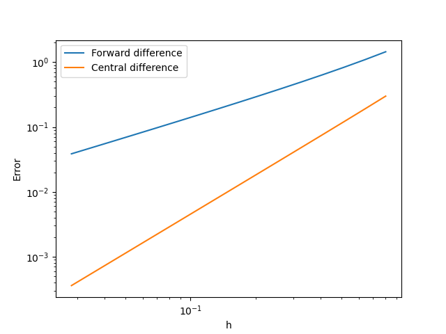
Let's explore the behavior of the accuracy of the forward difference formula and the central difference formula concerning the step size \(h\) by implementing an actual program. Similar to the previous example, a program to calculate the derivative value of the function \(f(x) = e^x\) at \(x=1\) is provided below.

using PyPlot

# Compute the derivative with the forward difference
function fdiff_forward(x, h)
    fx = exp(x)
    fx_ph = exp(x + h)
    dfdx = (fx_ph - fx) / h
    return dfdx
end

# Compute the derivative with the central difference
function fdiff_central(x, h)
    fx_ph = exp(x + h)
    fx_mh = exp(x - h)
    dfdx = (fx_ph - fx_mh) / (2.0 * h)
    return dfdx
end

# set the numerical parameters
x = 1.0
n = 16

# define the arrays
h = zeros(n)
dfdx_f = zeros(n)
dfdx_c = zeros(n)
error_f = zeros(n)
error_c = zeros(n)

for i in 1:n
    h[i] = 0.8 ^ i
    
# evaluate the derivative    
    dfdx_f[i] = fdiff_forward(x, h[i])
    dfdx_c[i] = fdiff_central(x, h[i])
    
# evaluate the error
    error_f[i] = abs.(dfdx_f[i] - exp(x))
    error_c[i] = abs.(dfdx_c[i] - exp(x))
end


#Plot the date
plt.plot(h, error_f, label="Forward difference")
plt.plot(h, error_c, label="Central difference")

plt.xscale("log")
plt.yscale("log")

plt.xlabel("h")
plt.ylabel("Error")
plt.legend()

plt.savefig("error_derivative.png")
plt.show()

Let's examine the Julia code provided above. The third line is a comment line starting with #, which doesn't have any impact on the program but serves as a reference for humans when reading the code. The fourth line defines the tdiff_forward(x, h) procedure using the function statement. The function block is closed with end at line 9. Procedures defined in this manner can be called within the program. This fourth line defines a function that computes the derivative value of a function using the forward difference formula and returns that value. Additionally, the function defined from line 12 defines a procedure for finding the derivative value using the central difference formula.

In line 24, the variable h is initialized as a Julia array of size n. The function zeros used here initializes the array by assigning 1 to all of its elements. Similarly, dfdx_f, dfdx_c, error_f, and error_f are initialized as arrays.

In the for loop starting at line 30, the derivative values of the function are calculated using the forward and central difference procedures defined above while varying the step size h[i].

In lines 34 and 35, the error is assessed by taking the difference between the calculated approximate value of the numerical derivative up to this point and the exact partial value.

The figure illustrates the plot generated by this code. Notably, the horizontal and vertical axes of the figure are logarithmic. Observing this, it becomes apparent that the error of the forward difference approximation (blue line) and the error of the central difference (orange line) are proportional to different powers of \(h\). This behavior aligns with the discussion on error magnitude above.

Lesson 1-3: Numerical Differentiation of Second-Order Derivatives

In the previous section, we numerically evaluated the first-order derivative using finite difference approximation. In this section, we will build upon the knowledge gained in the first-order derivative and explore how to numerically evaluate the second-order derivative. By employing the Taylor expansion equation, we can derive the following relationship: \[ \frac{f(x+h) - 2f(x) + f(x-h)}{h^2} = \frac{d^2f(x)}{dx^2} + \mathcal{O}(h^2). \] This equation can be utilized for the numerical evaluation of the second-order derivative, and the error is of the order of \(\mathcal{O}(h^2)\).

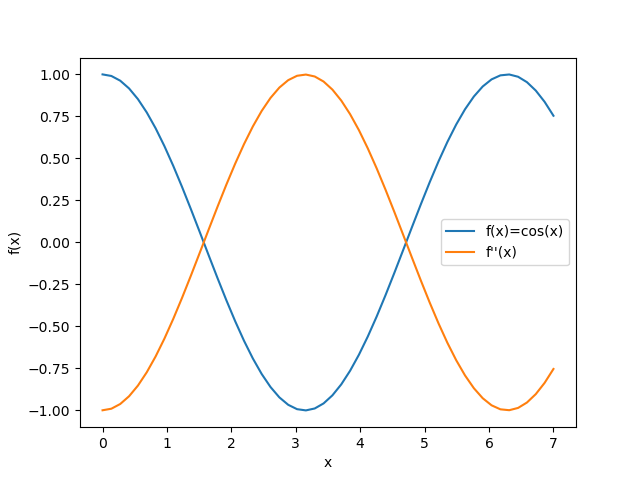
The provided Python code illustrates a program that numerically calculates the second derivative \(f''(x)\) of the function \(f(x) = \cos(x)\). Try writing a similar code on your own to acquaint yourself with second-order derivatives and Julia programming.

using PyPlot

function second_order_derivative_cos(x, h)
    fx = cos(x)
    fx_ph = cos(x + h)
    fx_mh = cos(x - h)
    d2fdx2 = (fx_ph - 2 * fx + fx_mh) / h^2
    return d2fdx2
end

h = 0.1
nx = 52
xini = 0.0
xfin = 7.0

x = range(xini, stop=xfin, length=nx)
fx = cos.(x)

d2fdx2 = second_order_derivative_cos.(x, h)

plt.plot(x, fx, label="f(x)=cos(x)")
plt.plot(x, d2fdx2, label="f''(x)")

plt.xlabel("x")
plt.ylabel("f(x)")
plt.legend()
plt.savefig("second_derivative_cos.png")
plt.show()

The above sample program provides the following figure showing \( f(x)=(\cos(x) \) and \(f''(x) \).