Lesson 3-1: Euler Method

Our exploration begins with the fundamental Euler method. Similar to our discussion of the forward difference formula in Section 1: Numerical Differentiation, we revisit the definition of the derivative. The derivative \(y'(x)\) of a function \(f(x)\) is defined as \begin{align} y'(x) = \lim_{h\rightarrow 0} \frac{y(x+h) - y(x)}{h}. \tag{2} \end{align} Assuming that \(h\) is sufficiently small in this equation, the derivative can be approximated using the forward difference formula as follows: \begin{align} y'(x) \approx \frac{y(x+h) - y(x)}{h}. \tag{3} \end{align} Rewriting this equation, we obtain \begin{align} y(x+h) \approx y(x) + y'(x)h. \tag{4} \end{align}

Examining equation \((4)\), the right side is expressed solely with the information of \(y(x)\) and \(y'(x)\) at \(x\), allowing us to approximately evaluate the value \(y(x+h)\) of the function at \(x+h\). By iteratively performing such operations, we can evaluate the value \(y(x)\) of the function at any variable \(x\). This numerical solution method for differential equations is known as the Euler method. The figure below visually illustrates the steps of the Euler method.

Below is a more detailed description of the Euler method procedure:

• First, set the initial condition \(y(x_0) = y_0\) in the differential equation \((1)\).
• Next, evaluate \(f(x_0, y(x_0))\) and determine the derivative value \(y'(x_0)\).
• Use the evaluated derivative value \(y'(x_0)\) to calculate the function value \(y(x_0 + h)\) at \(x_0 + h\) using formula \((4)\).
• Based on the calculated \(y(x_0 + h)\), compute the function value \(f(x_0 + h, y(x_0 + h))\) and determine the derivative value \(y'(x_0 + h)\) at \(x_0 + h\).
• Using the determined derivative value \(y'(x_0 + h)\), evaluate the function value \(y(x_0 + 2h)\) at \(x_0 + 2h\) using formula \((4)\).
• Repeat the same procedure as outlined below.

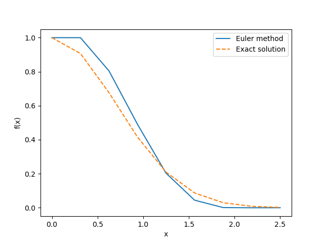
Following these steps enables the numerical solution of differential equations. As an exercise in numerically solving spherical differential equations using the Euler method, let's attempt to solve the following differential equation with the initial condition \(y(x=0)=1\): \begin{align} y'(x)=-2x y(x). \tag{5} \end{align} It's worth noting that the analytical solution of this differential equation is a Gaussian function, \(y(x)=e^{-x^2}\).

Below is an example Julia code. Each of you is encouraged to write your own code to solve the differential equation and observe how the accuracy of the obtained solution changes with varying step widths \(h\).

using PyPlot

# Define the derivative, dy/dx
function dydx(x, y)
    return -2.0 * x * y
end

# Euler method: compute y(x+h)
function euler_method(y, x, h)
    return y + dydx(x, y) * h
end

# Solve the differential equation from x=a to x=b with n discretized points
a = 0.0
b = 2.5
n = 8

h = (b - a) / n
x_values = range(a, stop=b, length=n+1)
y_values = zeros(n+1)
y_exact = zeros(n+1)

# Initial condition, y(a)=y_0
y_values[1] = 1.0
y_exact[1] = 1.0 

for i in 1:n
    y_values[i+1] = euler_method(y_values[i], x_values[i], h)
    y_exact[i+1] = exp(-x_values[i]^2)
end

# Plot the results
plt.plot(x_values, y_values, label="Euler method")
plt.plot(x_values, y_exact, label="Exact solution", linestyle="dashed")

plt.xlabel("x")
plt.ylabel("f(x)")
plt.legend()
plt.savefig("result_Euler.png")
plt.show()

The figure below shows the result obtained by the above source code.

Lesson 3-2: Predictor-Corrector Method

In the preceding section, we explored the Euler method as the most basic approach for solving differential equations. However, the Euler method is not commonly applied in computational science due to its limited accuracy. In this section, we introduce a method that offers increased accuracy while maintaining simplicity—the predictor-corrector method.

Additionally, a further rearrangement, similar to the Euler method, is performed resulting in \begin{align} y(x+h) \approx y(x) + \frac{dy\left(x+\frac{h}{2}\right)}{dx}h. \tag{7} \end{align}

Here, by replacing the derivative \( \frac{dy(x+h/2)}{dx} \) with the average of derivative values at \(x+h\) and \(x\), and utilizing the original differential equation \((1)\), we derive the following relationship. \begin{align} y(x+h) \approx y(x) + h\frac{f\left(x+h, y(x+h)\right) + f\left(x, y(x)\right)}{2}. \tag{8} \end{align} Although this formula offers a more accurate approximation than the Euler method, practical calculations pose challenges since information on the function's value \(y(x+h)\) at \(x+h\) is required when computing the right-hand side of Eq. \((8)\) to evaluate \(y(x+h)\) on the left side. To address this, a two-step procedure is employed for the practical evaluation of \(y(x+h)\) in Eq. \((8)\).

Firstly, in the initial step of the procedure (prediction step), we obtain the approximation of \(y(x)\) at \(x+h\) using the Euler method: \begin{align} \bar{y}(x+h) = y(x) + hf(x, y(x)). \tag{9} \end{align} Here, the approximated value is denoted as \(\bar{y}(x+h)\).

Subsequently, in the second step of the procedure (correction step), utilizing the obtained approximation \(\bar{y}(x+h)\), we evaluate the right side of equation \((7)\) and determine \(y(x+h)\) as follows: \begin{align} y(x+h) = y(x) + h\frac{f\left(x+h, \bar{y}(x+h)\right) + f\left(x, y(x)\right)}{2}. \tag{10} \end{align}

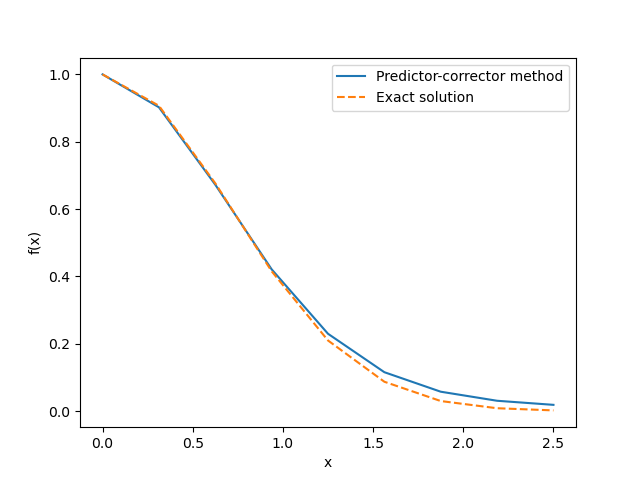
The two-step procedure for solving differential equations using Eq. \((9)\) and Eq. \((10)\) constitutes the numerical method known as the predictor-corrector method. To assess the accuracy of the predictor-corrector method in comparison to the Euler method, let's solve the differential equation \((5)\) using the predictor-corrector method and compare the results.

Below is an example Julia code demonstrating the solution of the differential equation \((5)\) using the predictor-corrector method.

using PyPlot

# Define the derivative, dy/dx
function dydx(x, y)
    return -2.0 * x * y
end

# Predictor-corrector method: compute y(x+h)
function pred_corr_method(y, x, h)
    y_bar = y + dydx(x, y) * h
    return y + 0.5 * h * (dydx(x, y) + dydx(x + h, y_bar))
end

# Solve the differential equation from x=a to x=b with n discretized points
a = 0.0
b = 2.5
n = 8

h = (b - a) / n
x_values = range(a, stop=b, length=n+1)
y_values = zeros(n+1)
y_exact = zeros(n+1)


# Initial condition, y(a)=y_0
y_values[1] = 1.0
y_exact[1] = 1.0
for i in 1:n
    y_values[i+1] = pred_corr_method(y_values[i], x_values[i], h)
    y_exact[i+1] = exp(-x_values[i+1]^2)
end

# Plot the results
plt.plot(x_values, y_values, label="Predictor-corrector method")
plt.plot(x_values, y_exact, label="Exact solution", linestyle="dashed")

plt.xlabel("x")
plt.ylabel("f(x)")
plt.legend()
plt.savefig("result_PredCorr.png")
plt.show()

The figure below displays the result obtained using the aforementioned source code.