Lesson 5-1: Monte Carlo Method Example (Computing Pi)

In this section, we will explore the Monte Carlo method. The Monte Carlo method is a computational approach that leverages random sampling to estimate solutions for complex problems, commonly encountered in physics, finance, and engineering. It models phenomena by generating numerous random samples, simulating the probabilities of various outcomes in processes influenced by random variables. By running multiple simulations, this method provides statistical approximations for problems too intricate for analytical solutions, with accuracy improving as the number of simulations increases.

The following Julia code demonstrates the application of the Monte Carlo method to estimate the value of Pi (π). This method relies on the principle of statistical probability and employs random sampling to obtain numerical results.

using Plots

# Number of random points to generate
n = 10000

# Initializing counters for points inside and outside the circle
num_inside_circle = 0
num_outside_circle = 0

# Arrays for storing points for plotting
x_inside = Float64[]
y_inside = Float64[]
x_outside = Float64[]
y_outside = Float64[]

# Generating random points and calculating Pi
for _ in 1:n
    x, y = rand(), rand()
    distance = x^2 + y^2

    if distance <= 1
        num_inside_circle += 1
        push!(x_inside, x)
        push!(y_inside, y)
    else
        num_outside_circle += 1
        push!(x_outside, x)
        push!(y_outside, y)
    end
end

# Estimating Pi
pi_estimate = 4 * num_inside_circle / n

# Plotting the points
plt.figure(figsize=(6,6))
plt.scatter(x_inside, y_inside, color="blue", s=1)
plt.scatter(x_outside, y_outside, color="red", s=1)
plt.title("Estimation of Pi using Monte Carlo Method: $(pi_estimate)")
plt.xlabel("X-axis")
plt.ylabel("Y-axis")
plt.savefig("pi_mc.png")
plt.show()

The provided Julia code utilizes the Monte Carlo method to estimate the value of π. This is achieved by generating random points within a unit square and determining the ratio of points inside a unit circle inscribed within the square. Here's a breakdown of the code:

1. using PyPlot: This line imports the PyPlot library, a Julia interface to the Matplotlib plotting library.
2. n = 10000: Sets the variable n to 10,000, representing the number of random points to generate.
3. Initializing counters and arrays:
   • num_inside_circle = 0 and num_outside_circle = 0: Counters tracking points inside and outside the unit circle.
   • x_inside, y_inside, x_outside, and y_outside: Arrays storing x and y coordinates of points for later plotting.
4. Generating random points and calculating Pi:
   • The for loop runs n times, generating random points (x, y) within the unit square (both x and y between 0 and 1).
   • Calculating the distance of each point from the origin using the formula distance = x^2 + y^2.
   • If distance is less than or equal to 1, the point is inside the unit circle, and counters are incremented, with coordinates stored in the corresponding arrays. If the distance is greater than 1, the point is outside the unit circle, and counters are updated.
5. Estimating Pi:
   • The variable pi_estimate is calculated using the formula pi_estimate = 4 * num_inside_circle / n
6. Plotting the points:
   • plt.figure(figsize=(6,6)): Sets the figure size.
   • scatter function: Creates a scatter plot of points inside (blue) and outside (red) the unit circle.
   • Title, x-axis label, and y-axis label are set.
   • savefig("pi_mc.png"): Saves the plot to a file named "pi_mc.png".
   • plt.show(): Displays the plot.

The employed Monte Carlo method is a probabilistic approach, and the precision of the estimation enhances as the number of randomly generated points increases. The accompanying plot vividly illustrates how random sampling effectively covers both the area of the unit square and the unit circle, elucidating the fundamental concept underlying Monte Carlo estimation.

The provided Julia code utilizes the Monte Carlo method to estimate the value of Pi by randomly generating points and determining their placement within or outside a unit circle. In this simulation, 10,000 points were generated.

The figure below visually represents the distribution of these points, showcasing points inside the circle in blue and points outside in red. This methodology capitalizes on the ratio of the area of a circle to the area of a square to approximate the value of Pi. Notably, the accuracy of this estimation increases with the number of points used in the simulation.

Lesson 5-2: Monte-Carlo Method for Integration

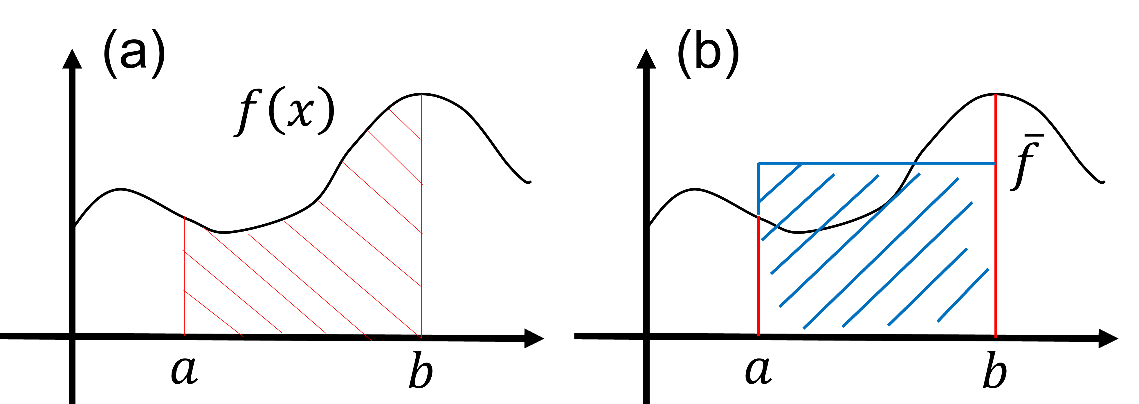
In this lesson, we delve into the Monte-Carlo method for integrating a function. Consider the integral: \begin{align} S = \int_a^b dx f(x). \tag{1} \end{align} The value of the integral, \(S\), corresponds to the red-shaded area in Figure (a) below. It's crucial to recognize that this integral value is also equivalent to the blue-shaded area in Figure (b), expressed as \begin{align} S = \int_a^b dx f(x) = (b-a) \times \bar{f}, \tag{2} \end{align} where \(\bar{f}\) is the average value of the function \(f(x)\) over the interval \((a \leq x \leq b)\). This observation implies that the integral \(S\) can be computed using the average value \(\bar{f}\) of the function \(f(x)\) within the integral range.

The Monte-Carlo method for integration relies on evaluating the average value, \( \bar f \). In the fundamental algorithm of the Monte-Carlo method for integrating Eq. (\(1\)), numerous random numbers \(x_i\) are generated within the interval \((a \le x \le b) \). The average value \( \bar f \) is then approximated as \begin{align} \bar f \approx \frac{1}{N} \sum_{i=1}^N f(x_i), \tag{3} \end{align} where \(N\) represents the total number of generated random numbers. Consequently, the integral of Eq. (\(1\)) can be approximated as \begin{align} S = \int_a^b dx f(x) = (b-a) \times \bar f \approx \frac{b-a}{N} \sum_{i=1}^N f(x_i) \tag{4} \end{align} using the set of random numbers \(\{x_i \}\) generated within the range \((a \le x \le b)\).

To become acquainted with the Monte-Carlo method, let's develop a Python program to evaluate the following integral: \begin{align} S = \int_0^1 dx \frac{4}{1+x^2}. \tag{5} \end{align} Analytically integrating Eq. (\(5\)) yields \(S = \pi\).

The following Python code exemplifies the implementation of the Monte Carlo method for estimating the value of \(S\) in Eq. (\(5\)).

# Number of random points to use for the Monte Carlo simulation
n = 10000

# Function to integrate
f(x) = 4.0 / (1.0 + x^2)

# Monte Carlo integration
integral = 0.0

for _ in 1:n
    integral += f(rand())
end

integral /= n

println("integral =", integral)

The provided Julia code serves as an illustration of utilizing the Monte Carlo method for numerical integration. Here's a detailed breakdown of its components and functionality:

1. n = 10000: This line initializes a variable n with the value 10000, representing the number of random points to be utilized in the Monte Carlo simulation.
2. f(x) = 4.0 / (1.0 + x^2): This line defines a function f(x) that calculates the value of the function \(f(x)=\frac{4.0}{1.0+x^2} \).
3. integral = 0.0: This line initializes a variable integral with the value 0.0. This variable accumulates the results of the Monte Carlo integration.
4. for _ in 1:n: This line starts a loop that iterates n times. The underscore _ is a placeholder for the loop variable, which is not used in the loop body.
5. integral += f(rand()): Within the loop, a random number is generated using rand(), and the value of the function f(x) at that random point is added to integral.
6. integral /= n: After the loop, the accumulated sum is divided by n to obtain the average value, representing the result of the Monte Carlo integration.
7. println("integral =", integral): Finally, the value of the integral is printed to the console using the println function. The result should represent an estimation of the integral using the Monte Carlo method.

In summary, this code provides an implementation of the Monte Carlo method for estimating the integral of a function within a defined interval. Specifically, it approximates the integral of 4/(1 + x^2) over the interval [0, 1], offering a means to estimate the value of π. The precision of this approximation hinges on the quantity of randomly generated points utilized.

Lesson 5-3: Monte-Carlo Method with General Distribution

In the preceding section, we explored the Monte-Carlo method using random numbers from a uniform distribution. In this section, we will delve into the application of the Monte-Carlo method utilizing a general distribution instead of a uniform distribution. Consider the following integral: \[ S = \int^{\infty}_{-\infty}dx f(x) w(x), \tag{6} \] where \( w(x) \) is a distribution function that is non-negative everywhere (i.e., \( w(x) \ge 0 \) for any \( x \)) and normalized (\( \int^{\infty}_{-\infty} dx w(x) = 1 \)). As long as the distribution function \( w(x) \) satisfies the non-negativity and normalization conditions, the integral in Eq. (6) can be evaluated using random numbers distributed according to \( w(x) \), as shown in the following summation: \[ S = \int^{\infty}_{-\infty}dx f(x) w(x) \approx \frac{1}{N}\sum^{N}_{i=1} f(x_i), \tag{7} \] where \( N \) is the number of random numbers, and \( \{x_i\} \) are the random numbers generated according to the probability distribution function \( w(x) \).

The Python random module offers support for various distributions, including uniform, exponential, and normal distributions. Additionally, it allows the generation of random numbers from arbitrary distributions, for instance, through methods like Metropolis sampling.

Here, we present an example of incorporating general distributions into the Monte-Carlo method. We will focus on computing the following integral, utilizing the normal distribution: \[ S=\int^{\infty}_{-\infty}dx x^2 \frac{1}{\sqrt{2\pi}} e^{-\frac{x^2}{2}}=1. \tag{7} \]

The Julia code below exemplifies the implementation of the Monte Carlo method to estimate the value of \( S \) in Equation (7).

# Number of random points to use for the Monte Carlo simulation
n = 10000

# Function to integrate
f(x) = x^2

# Monte Carlo integration
integral = 0.0

for _ in 1:n
    integral += f(randn())
end

integral /= n

println("integral =", integral)

Lesson 5-4: Importance Sampling

In this section, we explore a technique to enhance the convergence of Monte-Carlo sampling by utilizing a distribution function that aligns with the integrand. Consider modifying the integral as follows:

\begin{align} S=\int^{\infty}_{-\infty}dx f(x) =\int^{\infty}_{-\infty}dx \frac{f(x)}{w(x)}w(x), \tag{8} \end{align}

Here, \( w(x) \) is a distribution function satisfying the normalization condition \(\int^{\infty}_{-\infty}dx w(x)= 1\), and ensuring positivity \( w(x) > 0 \). Drawing upon the concepts from Lesson 5-3, we can evaluate the integral in Eq. (8) using Monte-Carlo sampling. This is done by sampling random numbers according to the distribution function \( w(x) \), as demonstrated in the following approximation:

\begin{align} S = \int^{\infty}_{-\infty}dx \frac{f(x)}{w(x)}w(x) \approx \frac{1}{N}\sum^N_i \frac{f(x_i)}{w(x_i)}, \tag{9} \end{align} where \( N \) represents the number of random numbers used, and \( \{x_i\} \) are the random numbers sampled from \( w(x) \).

The convergence speed of Monte-Carlo sampling, as depicted in Eq. (9), is influenced by the variability in the ratio \(\frac{f(x_i)}{w(x_i)}\). Consider a scenario where this ratio remains constant, regardless of \(x\). In such instances, even a single Monte-Carlo sample could result in a converged outcome. To expedite convergence in typical scenarios, it proves advantageous to select a distribution function \(w(x)\) closely resembling \(f(x)\). This resemblance minimizes fluctuations in the sampled values \(\frac{f(x_i)}{w(x_i)}\), facilitating quicker convergence.

Essentially, when the distribution function \(w(x)\) accentuates regions where the integrand \(f(x)\) is substantial, Monte-Carlo sampling experiences accelerated convergence. This strategy of choosing an optimal distribution function to enhance sampling efficiency is recognized as Importance Sampling.