In this section, we will explore the numerical solution of second-order ordinary differential equations expressed in the form: \begin{align} \frac{d^2y(x)}{dx^2} = f\left(x, y(x), \frac{dy(x)}{dx}\right). \tag{1} \end{align} Examples of such equations include Newton's equation of motion \(m\frac{d^2x(t)}{dt^2} = F(t)\).

Various methods exist for solving second-order ordinary differential equations. Here, to address these equations, we introduce the auxiliary variable \(s(x) = \frac{dy(x)}{dx}\). This allows us to transform equation \((1)\) into the following system of simultaneous first-order ordinary differential equations in two variables: \[ \frac{ds(x)}{dx} = f\left(x, y(x), s(x)\right), \tag{2} \] \[ \frac{dy(x)}{dx} = s(x). \tag{3} \] This transformation implies that second-order differential equations can be reformulated as a set of first-order ordinary differential equations. With this approach, the solution to the second-order differential equation becomes feasible by employing methods discussed in the previous section on First-order differential equations.

This section guides you through the numerical solution of second-order ordinary differential equations using Python. As an illustrative example, we consider the following second-order ordinary differential equation: \begin{align} \frac{d^2x(t)}{dt^2}=-x(t). \tag{4} \end{align} with initial conditions \(x(0)=0, \frac{dx(t)}{dt}=1\).

Introducing an auxiliary variable \(v(t)=\frac{dx(t)}{dt}\), equation \((4)\) can be reformulated as the following system of simultaneous differential equations: \[ \frac{dx(t)}{dt} = v(t), \tag{5} \] \[ \frac{dv(t)}{dt} = -x(t). \tag{6} \] Moreover, the initial condition \(x(0)=0, \frac{dx(0)}{dt}=1\) can be expressed as \(x(0)=0, v(0)=1\). Notably, the solution to this differential equation is \(x(t)=\sin(t)\) and \(v(t)=\cos(t)\).

The provided source code is written in Julia and is designed to solve the simultaneous first-order differential equations, Eqs. \((5)\) and \((6)\), employing the Euler method. To guide you in creating your own code to tackle similar simultaneous differential equations, consider the following reference code.

using PyPlot

function dxdt(v)
    return v
end

function dvdt(x)
    return -x
end

function euler_method(x, v, dt)
    x_new = x + dt * dxdt(v)
    v_new = v + dt * dvdt(x)
    return x_new, v_new
end

tini = 0.0
tfin = 10.0
n = 24
dt = (tfin - tini) / n

time = LinRange(tini, tfin, n + 1)
xt = zeros(n + 1)
vt = zeros(n + 1)
xt_exact = zeros(n + 1)
vt_exact = zeros(n + 1)

# Initial conditions
xt[1] = 0.0
vt[1] = 1.0
xt_exact[1] = 0.0
vt_exact[1] = 1.0

for i in 1:n
    xt[i + 1], vt[i + 1] = euler_method(xt[i], vt[i], dt)
    xt_exact[i+1]=sin(time[i+1])
    vt_exact[i+1]=cos(time[i+1])
end

# Plot the results
plt.plot(time, xt, label="x(t)")
plt.plot(time, vt, label="v(t)")
plt.plot(time, xt_exact, label="x(t): Exact", linestyle="dashed")
plt.plot(time, vt_exact, label="v(t): Exact", linestyle="dashed")

plt.xlabel("t")
plt.ylabel("x,v")
plt.legend()
plt.savefig("diff_2nd_Euler.png")
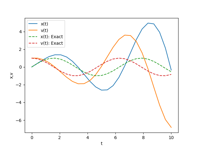
plt.show()

The figure below presents a comparison between the numerical solution obtained by executing the aforementioned source code and the exact solution. It is evident that the numerical solution obtained through the Euler method diverges significantly from the exact solution as time \(t\) progresses.

Building on our understanding from the previous section, we can enhance the accuracy of numerical solutions using methods such as the predictor-modifier method and the Runge-Kutta method. The provided sample source code illustrates an application of the predictor-modifier method to solve a set of differential equations, specifically Eqs. \((5)\) and \((6)\).

using PyPlot

function dxdt(v)
    return v
end

function dvdt(x)
    return -x
end

function pred_corr_method(x, v, dt)
    # Prediction
    x_pred = x + dt * dxdt(v)
    v_pred = v + dt * dvdt(x)

    # Correction
    x_new = x + 0.5 * dt * (dxdt(v) + dxdt(v_pred))
    v_new = v + 0.5 * dt * (dvdt(x) + dvdt(x_pred))
    return x_new, v_new
end

tini = 0.0
tfin = 10.0
n = 24
dt = (tfin - tini) / n

time = LinRange(tini, tfin, n + 1)
xt = zeros(n + 1)
vt = zeros(n + 1)
xt_exact = zeros(n + 1)
vt_exact = zeros(n + 1)

# Initial conditions
xt[1] = 0.0
vt[1] = 1.0
xt_exact[1] = 0.0
vt_exact[1] = 1.0

for i in 1:n
    xt[i + 1], vt[i + 1] = pred_corr_method(xt[i], vt[i], dt)
    xt_exact[i+1]=sin(time[i+1])
    vt_exact[i+1]=cos(time[i+1])
end


# Plot the results
plt.plot(time, xt, label="x(t)")
plt.plot(time, vt, label="v(t)")
plt.plot(time, xt_exact, label="x(t): Exact", linestyle="dashed")
plt.plot(time, vt_exact, label="v(t): Exact", linestyle="dashed")

plt.xlabel("t")
plt.ylabel("x,v")
plt.legend()
plt.savefig("diff_2nd_PredCorr.png")
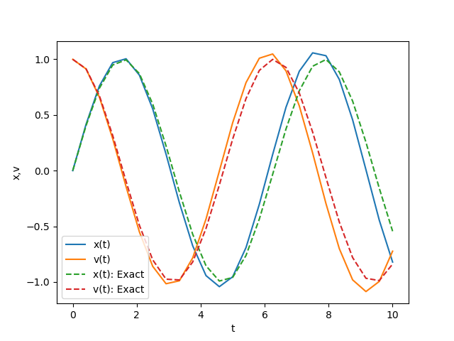
plt.show()

The figure below provides a comparison between the resultant numerical solution and the exact solution. Notably, the predictor-modifier method exhibits a significant enhancement in accuracy when contrasted with the Euler method.