<Previous Page: Numerical Solutions of Second-Order Differential Equations|

Lesson 5: The Monte Carlo Method

In this page, you will learn about the Monte Carlo method using Fortran.

If you are using a programming language other than Fortran, consider referring to the following pages:
Learning the Monte Carlo Method with Python
Learning the Monte Carlo Method with Julia

(lesson5_1.f90)

program main
  implicit none
  integer :: isample, nsample, ncount
  real(8) :: x1,x2,r

  nsample = 10000

  open(30,file="montecarlo.out")
  ncount = 0
  do isample = 1, nsample
     call random_number(x1)
     call random_number(x2)

     r = sqrt(x1**2+x2**2)
     if(r < 1d0)ncount = ncount + 1
     write(30,"(I10,2x,I10,2x,e26.16e3)")isample,ncount,4d0*ncount/dble(isample)
     
  end do
  close(30)

end program main

The provided Fortran code estimates the value of π using the Monte Carlo method. This is achieved by generating random points within a unit square and calculating the ratio of those points that fall inside a unit circle inscribed within the square. Here are the details of the code:

implicit none: This statement enforces explicit declaration of variables, improving code clarity and preventing potential issues related to undeclared variables.
Variable declarations:
- isample: A loop variable representing the current iteration of the Monte Carlo simulation.
- nsample: The number of Monte Carlo samples to be generated (set to 10,000).
- ncount: A counter for tracking the number of points within the unit circle.
- x1, x2: Variables to store random numbers generated between 0 and 1.
- r: The Euclidean distance from the point (x1, x2) to the origin.
open(30, file="montecarlo.out"): Opens a file named "montecarlo.out" for writing with unit number 30. This file will contain the results of the simulation.
do isample = 1, nsample: Begins a loop for the specified number of samples (nsample).
call random_number(x1) and call random_number(x2): Generates random numbers x1 and x2, both between 0 and 1.
r = sqrt(x1**2 + x2**2): Calculates the Euclidean distance from the point (x1, x2) to the origin.
if(r < 1d0) ncount = ncount + 1: Checks if the point (x1, x2) is inside the unit circle (distance from origin is less than 1). If true, increments the counter ncount.
write(30, "(I10,2x,I10,2x,e26.16e3)") isample, ncount, 4d0 * ncount / dble(isample): Writes formatted output to the file. This includes the current estimate of π based on the current simulation.
end do: Ends the loop.
close(30): Closes the output file.

In summary, this program conducts a Monte Carlo simulation by generating random points within a unit square and estimates π based on the proportion of points that fall inside a unit circle. The results of the simulation are recorded in a file named "montecarlo.out".

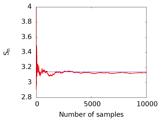
The following figure visually represents the value of π estimated using the aforementioned code as a function of the number of sampling points. As can be seen from the figure, the value converges to the accurate value of π (approximately 3.14) as the number of sampling points increases, demonstrating convergence in the limit of large sampling.

Figure: Result of the Euler methods for the second-order differential equation.

Lesson 5-2: The Monte Carlo Method for Integration

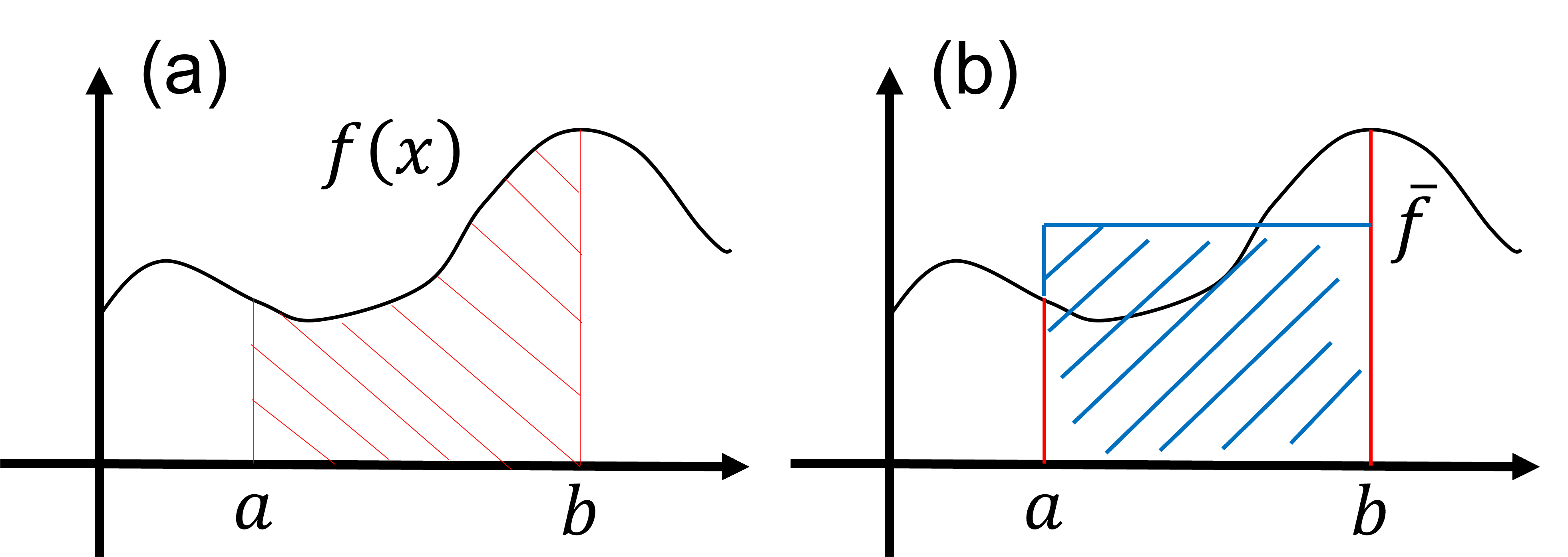
In this lesson, we explore the Monte Carlo method for the integration of functions. Consider the integral: \begin{align} S = \int_a^b dx f(x). \tag{1} \end{align} Here, the value of the integral \(S\) corresponds to the area painted red in the figure (a) below. Importantly, the value of this integral \(S\) is equivalent to the area painted blue in figure (b) as well. Specifically, it is expressed as: \begin{align} S = \int_a^b dx f(x) = (b-a) \times \bar{f}, \tag{2} \end{align} where \(\bar{f}\) is the average value of the function \(f(x)\) over the interval \((a \leq x \leq b)\). From this observation, it is suggested that the integral \(S\) can be calculated using the average value \(\bar{f}\) of the function \(f(x)\) within the integration range.

Figure: Schematic picture for numerical integral

The Monte Carlo method for integration involves calculating the average value \( \bar{f} \). In the core algorithm of Monte Carlo integration, many random numbers \(x_i\) are generated within the interval \((a \le x \le b) \) for integrating equation (\(1\)). The average value \( \bar{f} \) is then approximated as follows: \begin{align} \bar{f} \approx \frac{1}{N} \sum_{i=1}^N f(x_i), \tag{3} \end{align} where \(N\) represents the total number of random numbers generated. Thus, the integral of equation (\(1\)) is approximated as: \begin{align} S = \int_a^b dx \, f(x) = (b-a) \times \bar{f} \approx \frac{b-a}{N} \sum_{i=1}^N f(x_i) \tag{4} \end{align} using the set of random numbers \(\{x_i \}\) generated within the interval \((a \le x \le b)\).

To get accustomed to the Monte Carlo method, let's develop a Fortran program to evaluate the following integral: \begin{align} S = \int_0^1 dx \frac{4}{1+x^2}. \tag{5} \end{align} Analytically integrating equation (\(5\)) results in \(S = \pi\).

The Python code below is an example implementation that estimates the value of equation (\(5\)) using the Monte Carlo method.

(lesson5_2.f90)

program main
  implicit none
  integer :: isample, nsample
  real(8) :: x, f, s

  nsample = 10000

  s = 0d0
  open(30,file="pi_montecarlo.out")
  do isample = 1, nsample
     call random_number(x)
     f = 4d0/(1d0+x**2)
     s = s + f
     write(30,"(I10,2x,e26.16e3)")isample,s/isample
  end do
  close(30)

  
end program main

This Fortran program performs a Monte Carlo simulation to estimate the value of π. Here are the details of the code:

implicit none: This statement enforces explicit declaration of all variables, improving the clarity of the code and preventing potential issues related to undeclared variables.
Variable declarations:
- isample: A loop variable representing the current iteration of the Monte Carlo simulation.
- nsample: The number of Monte Carlo samples to be generated (set to 10,000).
- x: A variable to store random numbers generated between 0 and 1.
- f: A variable to store the function value based on the random number.
- s: A variable to accumulate the sum of function values.
nsample = 10000: Sets the number of Monte Carlo samples to 10,000.
s = 0d0: Initializes the variable s to zero. This variable is used to accumulate the sum of function values during the simulation.
open(30, file="pi_montecarlo.out"): Opens a file named "pi_montecarlo.out" for writing with unit number 30. This file will contain the results of the simulation.
do isample = 1, nsample: Begins a loop for the specified number of samples (nsample).
call random_number(x): Generates a random number x between 0 and 1.
f = 4d0 / (1d0 + x**2): Calculates the function value f based on the generated random number x. This function is for estimating π using the Monte Carlo method.
s = s + f: Accumulates the function value in the variable s.
write(30, "(I10,2x,e26.16e3)") isample, s/isample: Writes formatted output to the file. It includes the current sample number (isample) and the running average of the accumulated function values, which is used to estimate π.
end do: Ends the loop.
close(30): Closes the output file.

In summary, this program conducts a Monte Carlo simulation to estimate the value of π, where random points are generated, and their contributions to a specific mathematical function are accumulated. The running average of the accumulated values is used to approximate the value of π, and the results are written to a file named "pi_montecarlo.out".

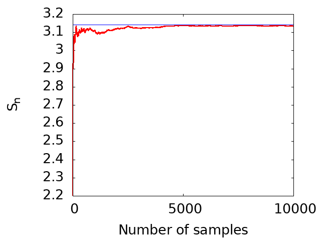
The following figure visually demonstrates the estimated values of π as a function of the number of sampling points, using the above code (lesson5_2.f90). As evident from the figure, the value converges to the accurate value of π (approximately 3.14) as the number of sampling points increases. This demonstrates convergence in the limit of large sampling.

<Previous Page: Numerical Solutions of Second-Order Differential Equations|

[Back to Fortran home]