Lesson 4: Numerical Solutions to Second-Order Ordinary Differential Equations

In this page, we will learn how to numerically solve second-order ordinary differential equations using Fortran.

If you are using a programming language other than Fortran, please also refer to the following pages:
Solving First-Order Ordinary Differential Equations in Python
Solving First-Order Ordinary Differential Equations in Julia

Second-order ordinary differential equations can generally be written in the following form: \[ \frac{d^2y(x)}{dx^2} =f\left (x,y(x), \frac{dy(x)}{dx} \right). \tag{1} \] Here, to solve second-order ordinary differential equations, we consider rewriting equation (1) as the following system of first-order differential equations: \[ v(x) = \frac{dy(x)}{dx}, \tag{2} \] \[ \frac{dv(x)}{dx} = f\left (x,y(x), v(x) \right). \tag{3} \] By introducing a new variable \(v(x)=dy(x)/dx\), we have rewritten the second-order differential equation as a system of two coupled differential equations. Such systems of first-order differential equations can be numerically solved using the methods learned in the previous page (Solving First-Order Ordinary Differential Equations). Furthermore, in general, an \(n\)th-order differential equation can be rewritten as a system of \(n\) coupled first-order ordinary differential equations.

Lesson 4-1: Euler's Method

Here, we first learn about solving second-order ordinary differential equations using Euler's method. The details of Euler's method are explained in the previous page (Solving First-Order Ordinary Differential Equations), so please refer to that for more information.

To learn about solving second-order ordinary differential equations using Euler's method, let's consider the Newtonian equation for a harmonic oscillator as an example. The Newtonian equation of motion for a harmonic oscillator can be written as follows: \[ m \frac{d^2x(t)}{dt^2}=-k x(t). \tag{4} \] Here \(m\) is the mass of the particle, and \(k\) is the spring constant. As discussed above, we consider rewriting this second-order differential equation into the following two coupled first-order ordinary differential equations: \[ v(t)=\frac{dx(t)}{dt}, \tag{5} \] \[ \frac{dv(t)}{dt} = -\frac{k}{m}x(t). \tag{6} \] Here, \(v(t)\) represents the velocity of the particle. Let's consider solving these coupled differential equations, equations (5) and (6), under the following initial conditions: \[ x(0)=0, \tag{7} \] \[ v(0)=1. \tag{8} \] The solution to these coupled differential equations can be found analytically and is given as follows: \[ x(t)=\sqrt{\frac{m}{k}} \sin \left [ \sqrt{\frac{k}{m}}t \right ], \tag{9} \] \[ v(t)=\cos \left [\sqrt{\frac{k}{m}}t \right ]. \tag{10} \]

The following program example solves the above differential equations (Newton's equations) using Euler's method.

(lesson4_1.f90)

program main
  implicit none
  real(8) :: k, m
  real(8) :: x, v, f
  real(8) :: x_new, v_new
  real(8) :: x_exact, v_exact
  real(8) :: t_fin, dt, t
  integer :: n, i

  n = 20
  t_fin = 10d0
  dt = t_fin/n

  k = 1d0
  m = 1d0


  x = 0d0
  v = 1d0

  open(20,file="newton_euler.out")

  t = 0d0
  x_exact = sin(t)
  v_exact = cos(t)

  write(20,"(5e16.6e3)")t,x,v,x_exact,v_exact


  do i = 0, n-1

     f = -k*x
     x_new = x + dt*v
     v_new = v + dt*f/m

     t = dt*(i+1)
     x_exact = sin(t)
     v_exact = cos(t)

     write(20,"(5e16.6e3)")t,x_new,v_new,x_exact,v_exact

     x = x_new
     v = v_new

  end do

  close(20)



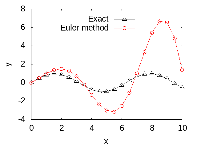
end program main

The following figure compares the numerical solution obtained by Euler's method as calculated by the above program with the analytical solution. You can see that the difference between the numerical and analytical solutions increases over time. This error is due to Euler's method being based on difference approximation, and it can be improved by reducing the time step size. However, the improvement in the accuracy of Euler's method by reducing the step size is very slow, so it is not often used in practical computations. In the next section, we will learn how to solve second-order differential equations (including Newton's equations) using the Predictor-Corrector method, which is an improvement over the Euler's method algorithm.

Numerical solution of Newton's differential equation with Euler's method

Lesson 4-2: Predictor-Corrector Method

Here, we attempt to solve the Newton equation, equation (1), using the Predictor-Corrector method. For details about the Predictor-Corrector method, please refer to "Numerical Solutions to First-Order Ordinary Differential Equations".

The following program example solves the above Newton equation using the Predictor-Corrector method.

(lesson4_2.f90)

program main
  implicit none
  real(8) :: k, m
  real(8) :: x, v, f
  real(8) :: x_pred, v_pred, f_pred
  real(8) :: x_new, v_new
  real(8) :: x_exact, v_exact
  real(8) :: t_fin, dt, t
  integer :: n, i

  n = 20
  t_fin = 10d0
  dt = t_fin/n

  k = 1d0
  m = 1d0


  x = 0d0
  v = 1d0

  open(20,file="newton_PredCorr.out")

  t = 0d0
  x_exact = sin(t)
  v_exact = cos(t)

  write(20,"(5e16.6e3)")t,x,v,x_exact,v_exact


  do i = 0, n-1

     f = -k*x
     x_pred = x + dt*v
     v_pred = v + dt*f/m
     f_pred = -k*x_pred
     
     x_new = x + dt*0.5d0*(v+v_pred)
     v_new = v + dt*0.5d0*(f+f_pred)/m

     t = dt*(i+1)
     x_exact = sin(t)
     v_exact = cos(t)

     write(20,"(5e16.6e3)")t,x_new,v_new,x_exact,v_exact

     x = x_new
     v = v_new

  end do

  close(20)



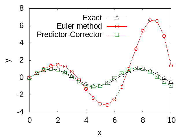
end program main

The figure below compares the numerical solution obtained by the Predictor-Corrector method using the above program with the numerical solution obtained by Euler's method, as well as with the analytical solution. From the figure, it can be seen that the accuracy of the Predictor-Corrector method is improved compared to the accuracy of Euler's method. Additionally, since the Predictor-Corrector method is also based on difference approximation, reducing the time step size can minimize the error.

Numerical solution of Newton's differential equation with Predictor-Corrector method

Lesson 4-3: Runge-Kutta Method

Here, we will implement a program to solve the Newton equation, equation (1), using the Runge-Kutta method. For details about the Runge-Kutta method, please refer to the previous discussion (Lesson 3).

The following program example solves the Newton equation using the Runge-Kutta method.

(lesson4_3.f90)

program main
  implicit none
  real(8) :: k, m
  real(8) :: x, v, f
  real(8) :: kx1,kx2,kx3,kx4
  real(8) :: kv1,kv2,kv3,kv4
  real(8) :: x_new, v_new
  real(8) :: x_tmp, v_tmp
  real(8) :: x_exact, v_exact
  real(8) :: t_fin, dt, t
  integer :: n, i

  n = 20
  t_fin = 10d0
  dt = t_fin/n

  k = 1d0
  m = 1d0


  x = 0d0
  v = 1d0

  open(20,file="newton_RungeKutta.out")

  t = 0d0
  x_exact = sin(t)
  v_exact = cos(t)

  write(20,"(5e16.6e3)")t,x,v,x_exact,v_exact


  do i = 0, n-1

     f = -k*x
     kx1 = v
     kv1 = f/m

     x_tmp = x + 0.5d0*dt*kx1
     v_tmp = v + 0.5d0*dt*kv1
     kx2 = v_tmp
     f = -k*x_tmp
     kv2 = f/m

     x_tmp = x + 0.5d0*dt*kx2
     v_tmp = v + 0.5d0*dt*kv2
     kx3 = v_tmp
     f = -k*x_tmp
     kv3 = f/m

     x_tmp = x + dt*kx3
     v_tmp = v + dt*kv3
     kx4 = v_tmp
     f = -k*x_tmp
     kv4 = f/m

     x_new = x + (dt/6d0)*(kx1+2d0*kx2+2d0*kx3+kx4)
     v_new = v + (dt/6d0)*(kv1+2d0*kv2+2d0*kv3+kv4)

     t = dt*(i+1)
     x_exact = sin(t)
     v_exact = cos(t)

     write(20,"(5e16.6e3)")t,x_new,v_new,x_exact,v_exact

     x = x_new
     v = v_new

  end do

  close(20)



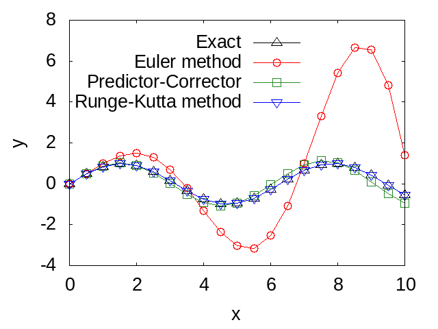
end program main

The figure below compares the numerical solution obtained by the Runge-Kutta method as calculated by the above program with the numerical solutions obtained by Euler's method and the Predictor-Corrector method, as well as with the analytical solution. From the figure, it is evident that the Runge-Kutta method provides higher precision calculations than both the Predictor-Corrector method and Euler's method.

Numerical solution of Newton's differential equation with Runge-Kutta method

[Back to Fortran Home]