Lesson 1: Numerical Differentiation

Lesson 1-1: Fundamentals of Numerical Differentiation: Approximation Using Difference Methods

Before numerically evaluating the derivative of a function, let's review the mathematical definition of differentiation. The derivative of the function \(f(x)\) is defined by the following equation: \[f'(x) = \lim_{h\rightarrow 0} \frac{f(x+h)-f(x)}{h}\] Based on this equation, the derivative of the function \(f'(x)\) can be approximated using a sufficiently small \(h\) as follows: \[f'(x) \approx \frac{f(x+h) - f(x)}{h}. \tag{1}\] This method of approximating the derivative using a finite size (but sufficiently small) width \(h\) is called finite difference method. The error in the approximation by the finite difference method can be evaluated using Taylor expansion, as follows. For instance, the Taylor expansion of the function \(f(x)\) is as follows. \[f(x+h) = f(x) + f'(x)h + O(h^2). \tag{2}\] Here, \(O(h^2)\) represents the error in truncating the Taylor series to a finite number of terms, consisting of terms of order \(h^2\) and higher. By transforming equation (\(2\)), we obtain the following equation. \[f'(x) = \frac{f(x+h)-f(x)}{h} + O(h).\] Therefore, the error in the finite difference approximation formula, equation (\(1\)), is proportional to \(h\). This is referred to as the \(O(h)\) [read as: order h] error. From this, we can see that the derivative value \(f'(x)\) can be accurately approximated using a sufficiently small \(h\).

By using Taylor expansion, it is also possible to create even more accurate approximation formulas. Here, let's consider the Taylor expansion up to the second order for the functions \(f(x+h)\) and \(f(x-h)\) as follows: \[f(x+h) = f(x) + f'(x)h + \frac{1}{2}f''(x)h^2 + O(h^3), \tag{3}\] \[f(x-h) = f(x) - f'(x)h + \frac{1}{2}f''(x)h^2 + O(h^3). \tag{4}\] By taking the difference between equations (\(3\)) and (\(4\)), the following approximation formula can be derived: \[f'(x) = \frac{f(x+h)-f(x-h)}{2h} + O(h^2). \tag{5}\] The error in this finite difference approximation formula, equation (\(5\)), is proportional to \(h^2\) and converges more rapidly to the exact derivative value in the limit of small \(h\) than the difference formula of equation (\(2\)). From this, it can be seen that for sufficiently small \(h\), equation (\(5\)) is a more accurate approximation formula than equation (\(2\)). A difference formula like equation (\(2\)) is called a forward difference formula, and a difference formula like equation (\(5\)) is called a central difference formula.

Computational Code for Numerical Differentiation Using Fortran

In this section, we will learn how to write Fortran code for numerical differentiation using the forward difference formula and the central difference formula. As a specific example, consider the differentiation of the exponential function, \(f(x)=e^x\) at \(x=0\). The following code calculates the derivative value, \(f'(0)\), varying the difference width, \(h\), and evaluates the error from the exact derivative value. The error in numerical differentiation is defined as the deviation from the exact derivative value: \( Error = \left|f'_{numerical}(0)-f'_{exact}(0) \right| \).

(lesson1_1.f90)

program main
  implicit none
  integer :: i, n
  real(8) :: ff_0, ff_p, ff_m, dfdx_f, dfdx_m, dfdx_e
  real(8) :: x, h

  x = 0d0
  dfdx_e = exp(x)
  
  h = 1d0
  
  n = 16
  open(20,file="fd_error.out")
  do i = 1, n
     ff_0   = exp(x)
     ff_p = exp(x+h)
     ff_m = exp(x-h)

     dfdx_f = (ff_p-ff_0)/h
     dfdx_m = (ff_p-ff_m)/(2d0*h)

     write(20,"(5e16.6e3)")h,dfdx_f,abs(dfdx_f - dfdx_e),dfdx_m,abs(dfdx_m - dfdx_e)
     
     h = h/2d0
  end do
  close(20)

  
end program main

In the above code, we are calculating the derivative value at \(x=0\). Therefore, in line 7 of the code, the variable x is assigned x=0. Also, in line 8, the exact derivative value of the function is calculated using dfdx_e = exp(x).

In line 13 of the code, the open statement is used to open a file for outputting the calculation results. Here, the file is opened using the following statement:

open(20,file="fd_error.out")

Here, the number 20 represents the device number, and the file name is assigned to this integer value (device number). Any natural number can be assigned as a device number, and it is used to refer to the file instead of its name. Thus, the open statement with file="fd_error.out" opens a file named fd_error.out and assigns it to the device number 20.

From line 14 in the code, a do loop begins. Within the do loop, the numerical differentiation is evaluated repeatedly while changing the step width \(h\). First, the interim values, \( \exp(x) \), \( \exp(x+h) \), \( \exp(x-h) \), are evaluated and assigned to the variables ff_0, ff_p, and ff_m, respectively. Then, the value of the forward difference formula, Eq. (\(1\)), is assigned to the variable dfdx_f. Similarly, the evaluation value by the central difference formula, Eq. (\(5\)), is assigned to the variable dfdx_m.

In line 22, the calculation results are outputted to the file using the following write statement:

write(20,"(5e16.6e3)")h,dfdx_f,abs(dfdx_f - dfdx_e),dfdx_m,abs(dfdx_m - dfdx_e)

Here, the calculation results are outputted to the file fd_error.out assigned to device number 20 using the write statement. This write statement defines the output format as "5e16.6e3". The first numeral 5 represents the output of five variables. The subsequent e denotes an exponential format for output. The following 16.6 means that the output will reserve 16 characters for each value and display 6 digits of the mantissa. The actual output can be seen to understand the meaning of this output.

At the end of this do loop, the step width h is halved, and the process is repeated from the top of the do loop.

After the predetermined number of iterations, the program exits the DO loop and ends with the close statement on line 26, closing the file.

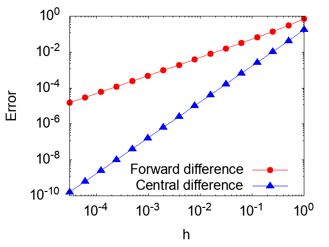
The figure below shows the results from fd_error.out outputted by the above program, illustrating the error in numerical differentiation as a function of the step width \(h\). As can be seen from the figure, the error in the differentiation evaluation using the central difference formula (Central difference) becomes significantly smaller as the step width \(h\) decreases, compared to the error from the forward difference formula (Forward difference). Therefore, as discussed above, it can be confirmed that in the limit of small \(h\), the error of the central difference formula converges to zero faster than the error of the forward difference.

Lesson 1-2: Numerical Handling of Second-Order Derivatives

As an extension of the first-order numerical differentiation covered in Lesson 1-1, we will learn about methods for numerically handling second-order derivatives. Similar to equations (\(3\)) and (\(4\)), consider the following Taylor expansions. \[f(x+h) = f(x) + f'(x)h + \frac{1}{2}f''(x)h^2 + \frac{1}{6}f^{(3)}(x)h^3 + O(h^4), \tag{6}\] \[f(x-h) = f(x) - f'(x)h + \frac{1}{2}f''(x)h^2 - \frac{1}{6}f^{(3)}(x)h^3 + O(h^4), \tag{7}\] Furthermore, using equations (6) and (7), the following relationship can be derived. \[f(x+h) -2 f(x) +f(x-h) = f''(x)h^2 +O(h^4). \tag{8}\] Further transforming the equation, the following can be obtained. \[f''(x) = \frac{f(x+h) -2 f(x) +f(x-h)}{h^2} +O(h^2). \tag{9}\] This equation is the difference formula for the second-order derivative, used for numerically evaluating the second-order derivative. Also, from the rightmost \(O(h^2)\), it can be understood that the error in the difference formula is proportional to \(h^2\).

As an example, we will look at a program that numerically calculates the second-order derivative of the trigonometric function \(f(x)=\sin(x)\). The trigonometric function can be differentiated analytically, and the second-order derivative of the function \(f(x)=\sin(x)\) is \(f''(x)=-\sin(x)\). To numerically evaluate this derivative, we consider a program using the difference formula, equation (7). Here, we evaluate the second-order part over one period of the trigonometric function (\( 0\le x \le 2 \pi \)).

(lesson1_2.f90)

program main
  implicit none
  integer :: i, n
  real(8) :: ff_0, ff_p, ff_m, d2fdx2
  real(8) :: x, h, x_i, x_f

  x_i = 0d0
  x_f = 2d0*3.14159d0
  
  n = 100
  h = (x_f - x_i)/n

  open(20,file="second_order_derivative_sin.out")
! second order derivative of sin(x)  
  do i = 0, n
     x = x_i + i*h

     ff_0 = sin(x)
     ff_p = sin(x+h)
     ff_m = sin(x-h)
     d2fdx2 = (ff_p - 2d0*ff_0 + ff_m)/h**2

     write(20,"(3e16.6e3)")x,d2fdx2,-sin(x)
  end do
  close(20)
  
end program main

In the above code, the second-order derivative of the trigonometric function \(f(x)=\sin (x)\) is evaluated over the range \(0 \le x \le 2\pi\). Here, the starting point of the evaluation range is set to x_i = 0d0, and the endpoint is set to x_f = 2d0*3.14159, where 3.14159 is an approximation of \(\pi\). Next, the interval between x_i and x_f is divided into n small intervals. The width of the small interval \(h\) is expressed by the formula: h = (x_f - x_i)/n. Inside the do loop of the above code, the second-order derivative value is evaluated by the difference formula, equation (\(7\)), and written to the output file second_order_derivative_sin.out. In the third column of this output file, the analytical evaluation value of the second-order derivative of the trigonometric function, -sin(x), is also outputted.

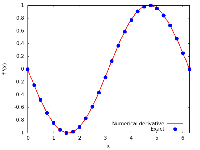
The figure below illustrates the results from second_order_derivative_sin.out outputted by the above program, comparing the values of the second-order derivative evaluated by the finite difference method with the exact values. It can be confirmed that the numerical differentiation successfully reproduces the exact values of the derivative.