Lesson 2: Numerical Integration

Lesson 2-1: Trapezoidal Rule and Numerical Integration

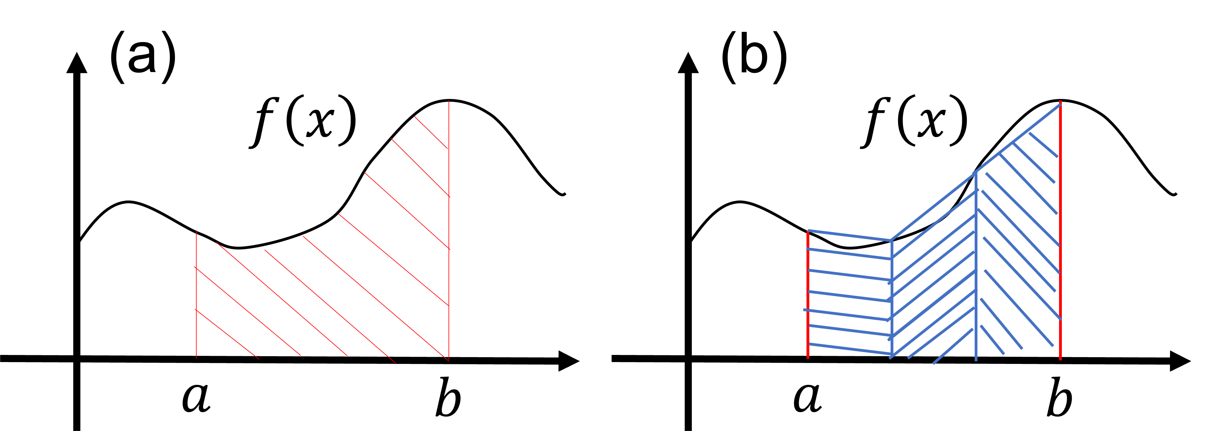
To evaluate integrals numerically, let's first review integrals. Here, we consider the integral of a function \(f(x)\) as follows: \[ S=\int^b_a dx f(x). \tag{1} \] The value of the integral \(S\) in equation (1) is known to be equal to the area of the part shaded with red diagonal lines in the figure below. Based on this fact, the integral value of formula \((1)\) can be approximated as the sum of the areas of multiple trapezoids. For instance, the area of the part shaded with red diagonal lines in figure (a) below can be approximated as the sum of the areas of the three trapezoids shaded with blue diagonal lines in figure (b). Assuming the integration interval \((a\le x \le b)\) is divided into three equal-width regions, the approximate value of the integral by the areas of the three trapezoids in figure (b) can be calculated as follows: \[ h = \frac{b-a}{3}, \tag{2} \] \[ S_3=\frac{f(a)+f(a+h)}{2}h+\frac{f(a+h)+f(a+2h)}{2}h +\frac{f(a+2h)+f(b)}{2}h. \tag{3} \] Here \(h\) represents the width of the divided intervals, and \(S_3\) represents the area of the region shaded with blue diagonal lines in figure (b). This formula can be further rewritten as follows: \[ S_3=h \times \left [ \frac{f(a)}{2}+f(a+h)+f(a+2h) + \frac{f(b)}{2} \right ]. \tag{4} \] This expression is in a convenient form for creating approximate formulas for integrals using a larger number of trapezoids, as we will see next.

In the above discussion, we considered evaluating the integral value of formula (\(1\)) using the approximation formula with three trapezoids as in formula (\(4\)). As expected from figure (b) above, increasing the number of divided intervals and using more trapezoids to approximate the area allows for a more accurate approximation of the integral value. For instance, if the integration interval \((a\le x \le b)\) is divided into \(N\) small intervals and the integral value of each small interval is approximated by the area of a trapezoid, the approximate value of the integral by the sum of the areas of \(N\) trapezoids can be expressed as follows: \[ h = \frac{b-a}{N}, \tag{5} \] \[ x_n = a + n\times h ~~~\rm{for}~~~ (0\le n \le N), \tag{6} \] \[ S_n = h\times \left [\frac{f(x_0)}{2} +f(x_1)+\cdots+f(x_{N-1})+\frac{f(x_N)}{2} \right ] \tag{7}. \] Here \(h\) represents the width of the divided small intervals, and \(x_n\) represents the coordinates of the \(n\)th grid point. Also, \(n\) represents an integer between \(0\) and \(N\). In this formula (\(7\)), the integral value of formula (\(1\)) is approximated by the areas of \(N\) trapezoids.

The approximation formula for the integral in formula (\(7\)) is known as the trapezoidal rule, and it becomes an exact formula for the integral value in the limit of a large number of divisions (\(N \rightarrow \infty\)).

Lesson 2-2: Writing Fortran Code Using the Trapezoidal Rule

Here, we will numerically evaluate the following integral using the trapezoidal rule (formula (\(7\))): \[ \int_0^1 dx \frac{4}{1+x^2}=\pi \tag{8}. \] The code below evaluates the integral by dividing the integration domain (\(0\le x \le 1\)) into \(N=20\) trapezoids. Also, explanations of the code are provided below it for your reference.

(lesson2_1.f90)

program main
  implicit none
  integer :: i, n
  real(8) :: a, b
  real(8) :: x, h, f, s


  n = 20

  a = 0d0
  b = 1d0
  h = (b-a)/n

  x = a
  f = 4d0/(1d0+x**2)
  s = 0.5d0*h*f
  do i = 1, n-1

     x = a + h*i
     f = 4d0/(1d0+x**2)
     s = s + h*f

  end do
  x = b
  f = 4d0/(1d0+x**2)
  s = s + 0.5d0*h*f

  write(*,*)"Result:"
  write(*,"(es26.16e3)")s
  
end program main

In the above Fortran code, the number of grid points is set to 20 with n=20 in line 8. Next, the integration range is defined in lines 10 and 11 as follows:

a = 0d0
b = 1d0 

After that, the width of the trapezoid is calculated in line 12 with:

h = (b-a)/n

In the block starting from line 14, the integral is evaluated using the trapezoidal rule (formula (\(7\))) by adding the values of the function to the variable s as follows:

  x = a
  f = 4d0/(1d0+x**2)
  s = 0.5d0*h*f
  do i = 1, n-1

     x = a + h*i
     f = 4d0/(1d0+x**2)
     s = s + h*f

  end do
  x = b
  f = 4d0/(1d0+x**2)
  s = s + 0.5d0*h*f

Finally, the result is output in the following block:

  write(*,*)"Result:"
  write(*,"(es26.16e3)")s

Is the result close to \(\pi=3.14159...\)? In the above code, a more accurate value can be obtained by setting a larger value for n. Let's check how the error as a function of n behaves.