Lesson 3:
Numerical Solutions to First-Order Ordinary Differential Equations

Lesson 3-1: Euler's Method

First, let's learn about the simplest calculation method called Euler's Method. To explain Euler's Method, let's review the differentiation of a function. The derivative of a function \(y(x)\) is defined as follows: \[ \frac{dy(x)}{dx}=\lim_{\Delta x \rightarrow 0}\frac{y(x+\Delta x)-y(x)}{\Delta x}. \tag{2} \] Based on this definition, we consider approximating the derivative using a sufficiently small \(\Delta x\). This kind of approximation is called a difference approximation. For more about difference approximation, see also the explanation in Numerical Differentiation. If we approximate formula (2) with a difference approximation, we can obtain the following approximate formula: \[ \frac{dy(x)}{dx}\approx \frac{y(x+\Delta x)-y(x)}{\Delta x}. \tag{3} \] This approximate formula (3) becomes exact in the limit \(\Delta x \rightarrow 0\). By substituting this formula (3) into the ordinary differential equation (\(1\)), we can create the following difference approximation for the ordinary differential equation: \[ y(x+\Delta x)=y(x)+\Delta f\left ( x,y(x) \right ). \tag{4} \] This difference approximation equation (4) plays a central role in solving differential equations using Euler's Method. As we will explain below, by repeatedly using this formula (4), we can sequentially determine the values of the function \(y(x)\).

Lesson 3-2: Specific Steps of Euler's Method

Here, we will look at the actual process of solving differential equations using Euler's Method. As an example, let's consider solving the differential equation (\(1\)) under the initial condition \(y(x_0)=y_0\). First, by applying formula (\(4\)) once at \( (x_0,y_0)\), we obtain the following equation. \[ y(x_0+\Delta x)=y_0 + \Delta x f(x_0,y_0). \tag{5} \] Here, let \(x_1 = x_0+\Delta x\) and \(y_1 = y(x_0+\Delta x)=y(x_1)\). Then, by further using formula (\(4\)), we get the next equation. \[ y(x_1+\Delta x)=y_1 + \Delta x f(x_1,y_1). \tag{6} \] Similarly, let \(x_2 = x_1+\Delta x\) and \(y_2 = y(x_1+\Delta x)=y(x_2)\). By repeating this operation, we can obtain the following recursive formula for a given data point \( (x_n, y_n)\). \[ y_n = y_{n-1} + \Delta x f(x_{n-1},y_{n-1}). \tag{7} \] This method is known as Euler's Method, and it is the simplest numerical solution method for differential equations. The figure below shows the process of sequentially solving differential equations using this Euler's Method.

Lesson 3-3: How to Write Fortran Code Using Euler's Method

Next, we will learn how to write Fortran code to solve first-order ordinary differential equations using Euler's Method. Here, as an example, we consider solving the following differential equation: \[ \frac{dy}{dx}=(y-1)y. \tag{8} \] Let's set the initial condition as \( y(0)=\frac{1}{10}\). This differential equation can be solved analytically, and its analytical solution is as follows: \[ y(x)=\frac{e^x}{9+e^x}. \tag{9} \] By substituting this equation (\(9\)) into equation (\(8\)), we can verify that it is indeed the solution to the differential equation.

The following program example solves the differential equation (\(8\)) using Euler's Method. Please refer to the explanations given below the code for your reference.

(lesson3_1.f90)

program main
  implicit none
  integer :: n, i
  real(8) :: x, f, y, y_new, dx, xf

  n = 8
  xf = 10d0
  dx = xf/n

  open(20,file="result_Euler.out")

  x = 0d0
  y = 1d0/10d0
  write(20,"(2e16.6e3)")x,y


  do i = 0, n-1

     x = dx*i
     f = (1d0-y)*y
     y_new = y + dx*f

     x = dx*(i+1)

     write(20,"(2e16.6e3)")x,y_new

     y = y_new

  end do

  close(20)

end program main

Lesson 3-3: How to Write Fortran Code Using Euler's Method

The code above solves the differential equation using Euler's method by dividing the range (\(0\le x \le 10\)) into 8 points. To achieve this, the code specifies the number of divisions with n=8 in line 6, and the endpoint for solving the differential equation with xf = 10d0 in line 7. From this information, the step size dx is calculated in line 8 with dx=xf/n.

In line 10 of the code, open(20,file="result_Euler.out") opens a file named result_Euler.out to prepare for outputting the results of the Euler's method calculation.

Lines 12 and 13 of the code set the initial condition \(y(0)=0\), and line 13 outputs the value of y at x=0 to the file result_Euler.out.

The DO loop starting from line 17 solves the differential equation using Euler's method formula, equation (7). First, lines 19 and 20 calculate the value of the function f at the i-th x coordinate (x_i), and line 21 calculates the value of y at the (i+1)-th x coordinate (y_i+1) using equation (7). Then, line 25 outputs the newly calculated (i+1)-th values (x_i+1, y_i+1) to the file with the write statement.

At the end of the DO loop, y=y_new assigns the newly calculated value of y (y_new) to the variable y, and the loop returns to the beginning. By repeating this procedure, the differential equation can be solved sequentially.

At the end of the code, close(20) closes the file "result_Euler.out" and ends the program.

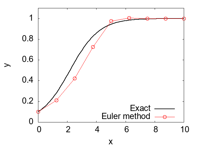
The figure below shows the numerical solution obtained with the Euler's method program (red line: Euler method) and the analytical solution (black line: Exact). You can see that there is a difference between the numerical solution of Euler's method and the analytical solution. This error in Euler's method originates from the difference approximation, and it is possible to reduce the error by using a smaller step size.

However, using a very small step size to obtain high precision solutions increases the computational cost. Instead of using smaller step sizes, it is also possible to enhance the accuracy of the numerical solution by using more sophisticated algorithms. In the next section, we will learn about an improved algorithm of Euler's method called the Predictor-Corrector method.

Lesson 3-4: Predictor-Corrector Method

As seen in the previous example, it is possible to numerically solve differential equations using Euler's method, but its accuracy is often insufficient for practical computations. Here, we will learn about the Predictor-Corrector method, which is a more accurate method than Euler's method. If we look closely at formula (3), we can see that Euler's method is based on forward difference. Therefore, let's consider creating an algorithm based on the more accurate central difference instead of the forward difference.

The approximation formula for differentiation using central difference is as follows: \[ \frac{dy \left (x +\frac{\Delta x}{2} \right )}{dx} \approx \frac{y(x+\Delta x) -y(x)}{\Delta x} \tag{10} \]

Using this formula (10), we can approximate differential equation (1) as follows. \[ \frac{y(x+\Delta x) -y(x)}{\Delta x} \approx \frac{dy \left (x +\frac{\Delta x}{2} \right )}{dx} = f\left ( x+\frac{\Delta x}{2},y \left (x+\frac{\Delta x}{2} \right ) \right) \tag{11} \].

Here, we further approximate the right-hand side of equation (11) as the average value of the function f at two points \(x\) and \(x+\Delta x \). \[ f\left ( x+\frac{\Delta x}{2},y \left (x+\frac{\Delta x}{2} \right ) \right) \approx \frac{f\left (x,y(x) \right) +f\left (x+\Delta x,y(x+\Delta x) \right) }{2} \tag{12} \]

Substituting equation (12) into equation (11) and rearranging, we can derive the following equation. \[ y(x+\Delta x)= y(x) + \frac{\Delta x}{2} \left [ f\left (x,y(x) \right) +f\left (x+\Delta x,y(x+\Delta x) \right) \right ] \tag{13} \] This equation (\(13\)) plays a central role in the Predictor-Corrector method. Moreover, since this equation (\(13\)) is based on the central difference approximation, it is a more accurate approximation than Euler's method, which is based on the forward difference approximation.

In principle, equation (13) can be used to numerically solve differential equation (1), but a problem arises when trying to write code using this equation. The problem is that to find \(y(x+\Delta x)\) on the left-hand side of equation (13), we need to use the value of \(y(x+\Delta x)\) itself on the right-hand side.

Thus, to find the value of \(y(x+\Delta x)\) using equation (13), we must already know that value. This characteristic of equation (13) is entirely different from the property of Euler's formula [equation (4)]. In the case of Euler's formula [equation (4)], the right-hand side is described using only known quantities, so there was no particular problem when determining the value of \(y(x+\Delta x)\) using Euler's method.

When actually performing numerical calculations using equation (13), instead of using equation (13) exactly, we approximate it to solve the differential equation numerically. To derive this approximation method, let's consider the following two-step process (known as the Predictor-Corrector method).

First, as the initial step, we predict the value of \(y(x+\Delta x)\) using Euler's method as follows: \[ y^{\rm{pred}}(x+\Delta x)=y(x)+f(x,y(x))\Delta x. \tag{14} \]

Next, as the second step (correction step), we use the predicted value \(y^{\rm{pred}}(x+\Delta x)\) as an approximation for \(y(x+\Delta x)\) in the right-hand side of equation (13): \[ y(x+\Delta x)= y(x) + \frac{\Delta x}{2} \left [ f\left (x,y(x) \right) +f\left (x+\Delta x,y^{\rm{pred}}(x+\Delta x) \right) \right ]. \tag{13} \]

In this way, the Predictor-Corrector method uses two steps, prediction and correction, to approximate equation (13).

To verify the accuracy of the Predictor-Corrector method, let's solve differential equation (8) using this method and compare the results with those obtained using Euler's method discussed earlier. Below is an example program for the Predictor-Corrector method for this comparison.

(lesson3_2.f90)

program main
  implicit none
  integer :: n, i
  real(8) :: x, f, y, y_new, dx, xf
  real(8) :: y_exact
  real(8) :: y_pred, f_pred


  n = 8
  xf = 10d0
  dx = xf/n

  open(20,file="result_PredictorCorrector.out")

  x = 0d0
  y = 0.1d0
  y_exact = exp(x)/(9d0+exp(x))
  write(20,"(3e16.6e3)")x,y,y_exact


  do i = 0, n-1

     x = dx*i
     f = (1d0-y)*y
     y_pred = y + dx*f

     f_pred = (1d0-y_pred)*y_pred
     y_new = y + dx*0.5d0*(f + f_pred)

     x = dx*(i+1)
     y_exact = exp(x)/(9d0+exp(x))

     write(20,"(3e16.6e3)")x,y_new,y_exact

     y = y_new

  end do

  close(20)

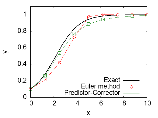
end program main

Using the above code, we can obtain a numerical solution to differential equation (8). The figure below shows a comparison between the results obtained by the Predictor-Corrector method, Euler's method, and the analytical solution. Here, both Euler's method and the Predictor-Corrector method use the same step size \(\Delta x \). As can be seen from the figure, the Predictor-Corrector method provides a more accurate numerical solution than Euler's method. As an exercise, try varying the step size in the above program and observe how the difference between the Predictor-Corrector method and the analytical solution changes.

Lesson 3-5: Runge-Kutta Method

The Predictor-Corrector method we learned in the previous section is a method that provides a more accurate numerical solution than Euler's method by taking two-step processes. This concept can be extended to conceive of an algorithm that provides even higher accuracy by taking multiple steps. The most commonly used high-accuracy algorithm is the Runge-Kutta method.

The Runge-Kutta method involves a four-step process to calculate four differential values, \(\frac{dy(x)}{dx} =f\left (x,y(x) \right )\), and from there, determines the next value of y (\(y(x+\Delta x)\)). To understand the Runge-Kutta algorithm, let's revisit Euler's method from the perspective of a multi-step method.

From the perspective of a multi-step method, Euler's method can be considered a method that finds the value of \(y(x+\Delta x)\) in the following one-step process: \[ k_1 = f(x, y(x)), \tag{15} \] \[ y(x+\Delta x) = y(x) + k_1 \times \Delta x . \tag{16} \] Equations (15) and (16) are equivalent to Euler's method [equation (4)] mentioned above.

The Runge-Kutta method can be viewed as an extension of Euler's method to a four-step process, and it finds the value of \(y(x+\Delta x)\) using the following algorithm: \[k_1 = f \left (x, y(x) \right ), \tag{17}\] \[k_2 = f\left (x+\frac{\Delta x}{2}, y(x)+ \frac{\Delta x}{2} k_1 \right ), \tag{18}\] \[k_3 = f\left (x+\frac{\Delta x}{2}, y(x)+ \frac{\Delta x}{2} k_2 \right ), \tag{19} \] \[k_4 = f\left (x+\Delta x, y(x)+k_3 \Delta x \right ), \tag{20}\] \[y(x+\Delta x) =y(x) + \Delta x \times \frac{k_1 + 2k_2 + 2k_3 + k_4}{6}. \tag{21} \] Using these equations (17-21) to solve differential equations with high accuracy is the (4th order) Runge-Kutta method.

The following program example numerically solves differential equation (8) using the Runge-Kutta method.

(lesson3_3.f90)

program main
  implicit none
  integer :: n, i
  real(8) :: x, f, y, y_new, dx, xf
  real(8) :: y_exact
  real(8) :: k1,k2,k3,k4,y_tmp


  n = 8
  xf = 10d0
  dx = xf/n

  open(20,file="result_RungeKutta.out")

  x = 0d0
  y = 0.1d0
  y_exact = exp(x)/(9d0+exp(x))
  write(20,"(3e16.6e3)")x,y,y_exact


  do i = 0, n-1

     x = dx*i

     k1 = (1d0-y)*y

     y_tmp = y+0.5d0*dx*k1
     k2 = (1d0-y_tmp)*y_tmp

     y_tmp = y+0.5d0*dx*k2
     k3 = (1d0-y_tmp)*y_tmp

     y_tmp = y+dx*k3
     k4 = (1d0-y_tmp)*y_tmp

     y_new = y + (dx/6d0)*(k1+2d0*k2+2d0*k3+k4)

     x = dx*(i+1)
     y_exact = exp(x)/(9d0+exp(x))

     write(20,"(3e16.6e3)")x,y_new,y_exact

     y = y_new

  end do

  close(20)

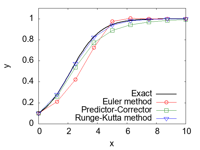
end program main

Using the above program, we can numerically solve differential equation (8). The figure below shows a comparison of the numerical solution obtained by the Runge-Kutta method with those obtained by the Predictor-Corrector method, Euler's method, and the analytical solution. As can be seen from the figure, the Runge-Kutta method very accurately solves the differential equation.