Lesson 2: Numerical Integration

On this page, we will learn about numerical integration, a method to evaluate integrals numerically using Python.

If you are using a programming language other than Python, you might find the following pages useful:
Numerical Integration in Julia
Numerical Integration in Fortran

Lesson 2-1: The Trapezoidal Rule and Numerical Integration

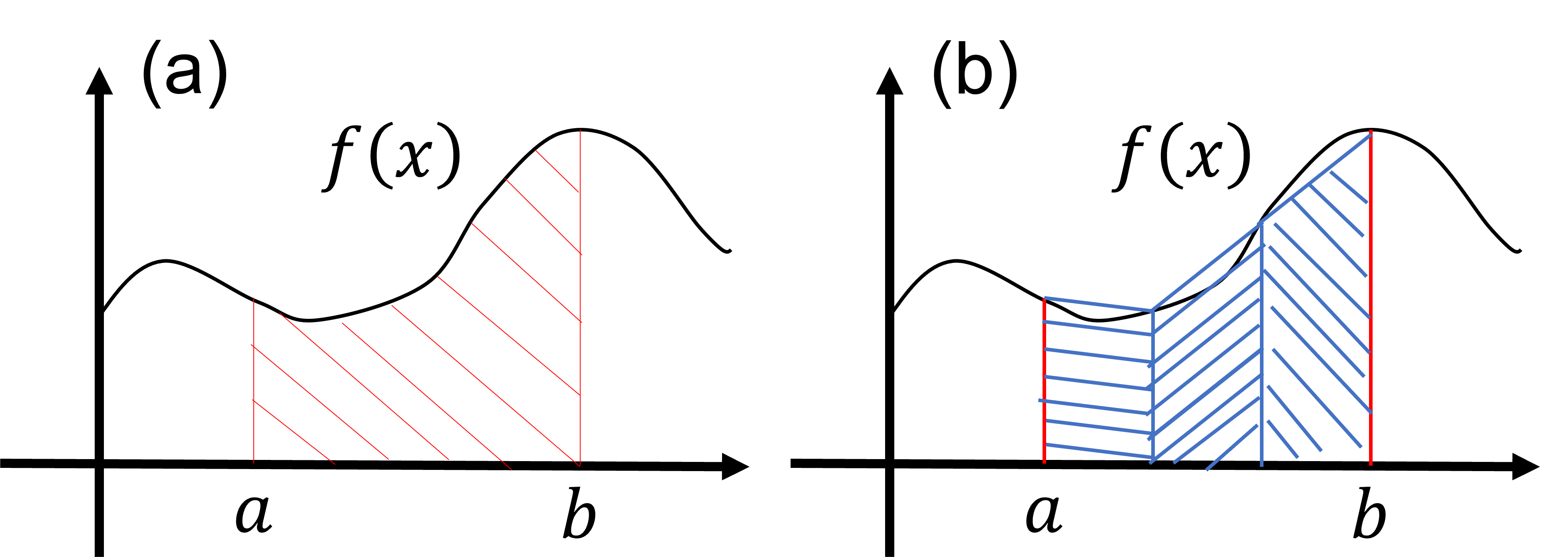
In this section, we learn about numerical integration, a method for evaluating the integral of a function numerically. First, consider the integral of a function \(f(x)\) as follows: \[ S=\int^{b}_{a} dx f(x). \tag{1} \] The value of the integral \(S\) in equation (1) is equal to the area filled by the red diagonal lines in the figure below (a).

Based on this fact, we consider approximating the integral in equation (1) as the sum of multiple trapezoids. For example, the area filled by the red diagonal lines in figure (a) can be approximated by the sum of the areas of three trapezoids filled by the blue diagonal lines in figure (b).

If we assume that the integration interval \((a\le x \le b)\) is divided into three regions of equal width, the approximate value of the integral by the area of the three trapezoids in figure (b) can be calculated as follows: \[ h = \frac{b-a}{3}, \tag{2} \] \[ S_3=\frac{f(a)+f(a+h)}{2}h+\frac{f(a+h)+f(a+2h)}{2}h +\frac{f(a+2h)+f(b)}{2}h. \tag{3} \] Here, \(h\) represents the width of the divided interval, and \(S_3\) represents the area of the region filled by the blue diagonal lines. This equation can be rewritten as follows: \[ S_3=h \times \left [ \frac{f(a)}{2}+f(a+h)+f(a+2h) + \frac{f(b)}{2} \right ]. \tag{4} \] This expression is convenient for creating an approximation of the integral by a larger number of trapezoids, as we will see next.

Conceptual diagram of numerical integration using the trapezoidal rule

In the above discussion, we considered evaluating the integral value in equation (1) using an approximate formula with three trapezoids as in equation (4). As expected from figure (b) above, by increasing the number of intervals divided and using more trapezoids to approximate the area, we can approximate the integral value more accurately.

Here, more generally, we consider dividing the integration interval (\(a \le x \le b\)) into N parts. Then, the width of each division \(\Delta x\) is defined by \(\Delta x =(b - a)/N\). Let's rewrite the integral S as the sum of the integrals of each divided interval as follows: \begin{align} S&=\int^{a}_{b} dx f(x) \\ &= \int^{a+\Delta x}_{a} dx f(x)+ \int^{a+2\Delta x}_{a+\Delta x} + \int^{a+3\Delta x}_{a+2\Delta x} dx f(x) + \cdots + \int^{b}_{a+(N-1)\Delta x} dx f(x) \\ &=\sum^{N-1}_{j=0} \int^{a + (j+1)\Delta x}_{a + j\Delta x} dx f(x) \tag{5} \end{align}

Assuming that the division width \(\Delta x\) is sufficiently small, the integrand \(f(x)\) can be approximated as the average of the values at the endpoints of each integration interval. In other words, equation (5) can be approximated as follows. \begin{align} S&=\sum^{N-1}_{j=0} \int^{a + (j+1)\Delta x}_{a + j\Delta x}f(x)dx \nonumber \\ &\approx \sum^{N-1}_{j=0} \int^{a + (j+1)\Delta x}_{a + j\Delta x} \frac{f \left ( a + (j+1)\Delta x \right )+f\left (a + j\Delta x \right )}{2} \nonumber \nonumber \\ &= \sum^{N-1}_{j=0}\frac{f \left ( a + (j+1)\Delta x \right )+f\left (a + j\Delta x \right )}{2} \int^{a + (j+1)\Delta x}_{a + j\Delta x}dx \nonumber \\ &= \sum^{N-1}_{j=0} \frac{f \left ( a + (j+1)\Delta x \right )+f\left (a + j\Delta x \right )}{2} \Delta x \nonumber \\ &= \frac{f(a)}{2}\Delta x + \left [ \sum^{N-1}_{j=1} f(a + j\Delta x) \Delta x \right ] + \frac{f(b)}{2}\Delta x \tag{6} \end{align}

The approximate formula in equation (6) is called the Trapezoidal Rule or Trapezoidal Formula, and this name comes from approximating the integral value as the sum of the areas of trapezoids. Also, by setting N=3 in equation (6), you can see that it reproduces the approximate formula for the integral using three trapezoids as in equation (3).

This equation (6), in the limit of a large number of divisions (\(N\rightarrow \infty\), \(\Delta x \rightarrow 0\)), the Trapezoidal Rule from equation (3) will match the exact integral value \(S\).

As an exercise, let's evaluate the following integral using the Trapezoidal Rule. \begin{align} S=\int^1_0 dx \frac{4}{1+x^2}=\pi . \end{align} Below is Python code for numerically evaluating the above integral. To become familiar with numerical integration and Python programming, try evaluating the integral using your own code by referring to the sample code.

(lesson2_1.py)

 import numpy as np
 
 # define your function
 def my_func(x):
     return 4.0/(1.0+x**2)
 
 # integrate the function from a to b with n points
 def integrate(f,a,b,n):
     h = (b-a)/n
 
     s = (f(a)+f(b))/2.0
     for i in range(1,n):
         x = a + i*h
         s += f(x)
 
     s = s*h
     return s
 
 
 
 a = 0.0
 b = 1.0
 n = 64
 
 num_integral = integrate(my_func,a,b,n)
 
 print('num. integral = ',num_integral)
 print('pi            = ',np.pi)

[Back to Python]