Lesson 4: Solving Second-Order Ordinary Differential Equations

On this page, we will learn about solving second-order ordinary differential equations numerically using Python.

If you are using a programming language other than Python, consider referring to the following pages:
Solving Second-Order Ordinary Differential Equations with C/C++
Solving Second-Order Ordinary Differential Equations with Julia
Solving Second-Order Ordinary Differential Equations with Fortran

In this section, we will learn about solving second-order ordinary differential equations that can generally be written in the following form: \begin{align} \frac{d^2y(x)}{dx^2}=f\left (x,y(x), \frac{dy(x)}{dx} \right). \tag{1} \end{align} Such second-order differential equations include Newton's equation of motion \(m\frac{d^2x(t)}{dt^2}=F(t)\).

There are several methods to solve second-order differential equations. Here, we introduce an auxiliary variable \(s(x)=\frac{dy(x)}{dx}\) to transform equation (1) into a system of two first-order ordinary differential equations as follows: \[ \frac{ds(x)}{dx} =f\left (x,y(x), s(x)\right), \tag{2} \] \[ \frac{dy(x)}{dx} =s(x). \tag{3} \] This demonstrates that a second-order differential equation can be rewritten as a pair of first-order differential equations. The first-order differential equations introduced by such transformation can be solved using the numerical solution methods for first-order differential equations learned in the previous section, Solving First-Order Differential Equations. Thus, second-order differential equations can be solved by converting them into a system of first-order differential equations and using methods for solving first-order differential equations.

On this page, we will learn about numerical solutions for second-order differential equations by writing Python code to solve the following second-order differential equation as a concrete example: \begin{align} \frac{d^2x(t)}{dt^2}=-x(t). \tag{4} \end{align} Here, the initial conditions are \(x(0)=0, \dot x(t)=1\).

By introducing the auxiliary variable \(v(t)=\frac{dx(t)}{dt}\), equation (4) can be rewritten as the following system of differential equations: \[ \frac{dx(t)}{dt} =v(t), \tag{5} \] \[ \frac{dv(t)}{dt} =-x(t). \tag{6} \] Furthermore, the initial conditions \(x(0)=0, \dot x(0)=1\) can be rewritten as \(x(0)=0, v(0)=1\).

Lesson 4-1: Euler's Method

The source code below uses Euler's method to solve the system of first-order differential equations, equations (5) and (6), using Python. Use this source code as a reference to create your own code for solving systems of differential equations.

(lesson4_1.py)

 from matplotlib import pyplot as plt
 import numpy as np
 
 def dxdt(v):
     return v
 
 def dvdt(x):
     return -x
 
 def euler_method(x,v,dt):
     x_new = x + dt*dxdt(v)
     v_new = v + dt*dvdt(x)
     return x_new, v_new
 
 tini = 0.0
 tfin = 10.0
 n = 24
 dt = (tfin - tini)/n
 
 time = np.linspace(tini,tfin,n+1)
 xt = np.zeros(n+1)
 vt = np.zeros(n+1)
 
 # Initial conditions
 xt[0] = 0.0
 vt[0] = 1.0
 
 for i in range(n):
     xt[i+1], vt[i+1] = euler_method(xt[i],vt[i],dt)
 
 
 # Plot the results
 plt.plot(time, xt, label='x(t)')
 plt.plot(time, vt, label='v(t)')
 plt.plot(time, np.sin(time), label='x(t): Exact', linestyle='dashed')
 plt.plot(time, np.cos(time), label='v(t): Exact', linestyle='dashed')
 
 plt.xlabel('t')
 plt.ylabel('x,v')
 plt.legend()
 plt.savefig("diff_2nd_Euler.png")
 plt.show()

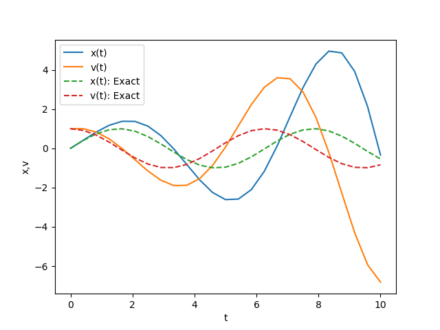
The figure below shows a comparison between the numerical solution obtained by executing the above source code and the exact solution. The numerical solution obtained by Euler's method deviates significantly from the exact solution as time \(t\) progresses.

Figure: Result of the Euler methods for the second-order differential equation.

As we learned in the previous section, the accuracy of numerical solutions can be improved by using methods such as the Predictor-Corrector method or the Runge-Kutta method. The sample source code below shows an example of code for solving the series of differential equations, equations (5) and (6), using the Predictor-Corrector method.

(lesson4_2.py)

 from matplotlib import pyplot as plt
 import numpy as np
 
 def dxdt(v):
     return v
 
 def dvdt(x):
     return -x
 
 def pred_corr_method(x,v,dt):
 # prediction
     x_pred = x + dt*dxdt(v)
     v_pred = v + dt*dvdt(x)
     
 # correction
     x_new = x + 0.5*dt*(dxdt(v)+dxdt(v_pred))
     v_new = v + 0.5*dt*(dvdt(x)+dvdt(x_pred))
     return x_new, v_new
 
 tini = 0.0
 tfin = 10.0
 n = 24
 dt = (tfin - tini)/n
 
 time = np.linspace(tini,tfin,n+1)
 xt = np.zeros(n+1)
 vt = np.zeros(n+1)
 
 # Initial conditions
 xt[0] = 0.0
 vt[0] = 1.0
 
 for i in range(n):
     xt[i+1], vt[i+1] = pred_corr_method(xt[i],vt[i],dt)
 
 
 # Plot the results
 plt.plot(time, xt, label='x(t)')
 plt.plot(time, vt, label='v(t)')
 plt.plot(time, np.sin(time), label='x(t): Exact', linestyle='dashed')
 plt.plot(time, np.cos(time), label='v(t): Exact', linestyle='dashed')
 
 plt.xlabel('t')
 plt.ylabel('x,v')
 plt.legend()
 plt.savefig("diff_2nd_PredCorr.png")
 plt.show()

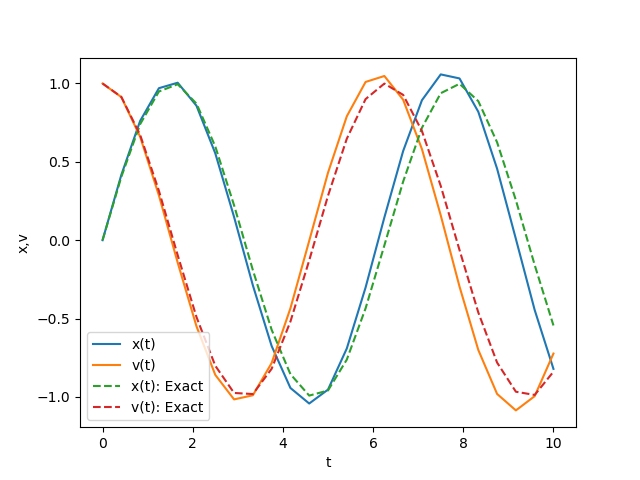
The figure below shows a comparison between the numerical solution obtained and the exact solution. The Predictor-Corrector method can significantly improve accuracy compared to Euler's method.

Figure: Result of the predictor-corrector method for the second-order differential equation.

[Back to Python]