Lesson 1: Numerical Differentiation

Lesson 1-1: The Difference Method (Forward Difference)

To consider methods for performing numerical differentiation, let's first review the mathematical definition of differentiation. The differentiation of a function \(f(x)\) is defined as follows. \[f'(x)=\lim_{h\rightarrow 0} \frac{f(x+h)-f(x)}{h}.\]

Using this definition of differentiation, we approximate the differentiation \(f'(x)\) of the function \(f(x)\) using a sufficiently small width \(h\) as follows. \[ f'(x)\approx \frac{f(x+h)-f(x)}{h}. \tag{1}\] This approximation of differentiation using a finite width \(h\) is called a finite difference approximation, or simply a difference approximation. In particular, the formula using the value \(f(x+h)\) moved forward, like in equation (1), is called the forward difference formula.

To verify the accuracy of the difference approximation, let's evaluate the differentiation of the function \(f(x)=e^x\) at \(x=1\) using equation (1) and compare it with the exact value \(f'(1)=e^1=e\). Let's look at the source code below.

(lesson1_1.py)

 import numpy as np
 
 x = 1.0
 h = 0.1
 
 f0 = np.exp(x)
 fp = np.exp(x+h)
 
 dfdx = (fp-f0)/h
 
 print('h=',h)
 print('dfdx=',dfdx)
 print('Error=',dfdx-np.exp(1.0))

Below is an explanation of the overview of the source code mentioned above. In the first line, the module numpy is imported using import numpy as np, preparing to use numpy's mathematical functions. By adding as np during import, the shorthand name np for numpy is defined, allowing us to call numpy as np.

In the third and fourth lines of the code, the differential value at \(x=1\) is set to be evaluated using the difference formula (1) with a step width \(h=0.1\), by setting the values with x = 1.0 and h = 0.1.

In the sixth and seventh lines of the code, the value of the function at \(x\) and \(x+h\) is calculated using the exponential function np.exp() of numpy, and stored in the variables f0 and fp, respectively. In the ninth line, the differential value is approximately evaluated using the forward difference formula. Additionally, in the twelfth and thirteenth lines, the difference between the approximate value of the differentiation obtained by the above calculation and the exact value of the differentiation is output.

Run the above program to check whether the differentiation is well approximated by the difference approximation. Also, see how the accuracy of the approximation changes by varying the step width \(h\).

Lesson 1-2: The Difference Method and Its Accuracy (Central Difference Approximation)

In the previous section, we learned about the finite difference method as a way to approximate differentiation. From the definition of differentiation, as the width \(h\) becomes smaller, the approximation becomes more precise, so it is expected that the approximation error also decreases with \(h\).

Here, let's evaluate the size of this error using Taylor expansion. First, consider the following Taylor expansion: \[f(x+h)=f(x)+f'(x)h+\mathcal{O}(h^2). \tag{2}\] Here, \(O(h^2)\) represents the terms of order \(h^2\) and higher, indicating the error from truncating the Taylor series at a finite order. By rearranging equation (2), we obtain the following expression. \[f'(x)=\frac{f(x+h)-f(x)}{h}+\mathcal{O}(h).\]

Therefore, the error in the forward difference formula (1) is \(\mathcal{O}(h)\), and the error in the approximation is proportional to \(h\) in the limit of small \(h\).

Moreover, using Taylor expansion, it is possible to create a more accurate difference approximation formula. Here, let's consider two Taylor expansions as follows: \[ f(x+h)=f(x)+f'(x)h+\frac{1}{2}f''(x)h^2 + \mathcal{O}(h^3),\] \[ f(x-h)=f(x)-f'(x)h+\frac{1}{2}f''(x)h^2 + \mathcal{O}(h^3).\] By taking the difference of these two equations and dividing by \(h^2\), we can create the following difference formula. \[ f'(x)=\frac{f(x+h)-f(x-h)}{2h}+\mathcal{O}(h^2). \tag{3} \] This difference formula is called the central difference formula, taking symmetric differences in both positive and negative directions. The error term is \(\mathcal{O}(h^2)\), indicating an error of order \(h^2\).

Let's write an actual program to verify how the accuracy of the forward difference formula and the central difference formula behaves with respect to the step width \(h\). Similar to the above example, a Python program that finds the derivative value of the function \(f(x)=e^x\) at \(x=1\) is shown below.

(lesson1_2.py)

 from matplotlib import pyplot
 import numpy as np
 
 
 # Compute the derivative with the forward difference
 def fdiff_forward(x,h):
     fx = np.exp(x)
     fx_ph = np.exp(x+h)
     dfdx = (fx_ph-fx)/h
     return dfdx
 
 # Compute the derivative with the central difference
 def fdiff_central(x,h):
     fx_ph = np.exp(x+h)
     fx_mh = np.exp(x-h)
     dfdx = (fx_ph-fx_mh)/(2.0*h)
     return dfdx
 
 # set the numerical parameters
 x = 1.0
 n = 16
 
 # define the arrays
 h = np.zeros(n)
 dfdx_f = np.zeros(n)
 dfdx_c = np.zeros(n)
 
 for i in range(n):
     h[i] = 0.8**i
     dfdx_f[i] = fdiff_forward(x,h[i])
     dfdx_c[i] = fdiff_central(x,h[i])
 
 # evaluate the error
 error_f = np.abs(dfdx_f - np.exp(x))
 error_c = np.abs(dfdx_c - np.exp(x))
 
 
 # Plot the date
 pyplot.plot(h, error_f, label="Forward difference")
 pyplot.plot(h, error_c, label="Central difference")
 
 pyplot.xscale('log')
 pyplot.yscale('log')
 
 pyplot.xlabel('h')
 pyplot.ylabel('Error')
 pyplot.legend()
 
 pyplot.savefig("error_derivative.png")
 pyplot.show()

Let's look at the above Python program.

Line 5 is a comment line that starts with #, which does not affect the program but is written to help those reading the program understand it better. Line 6 defines a procedure fdiff_forward(x,h) using the def statement. Procedures defined with a def statement can be called from within the program. The block representing this procedure is denoted by indentation. The function fdiff_forward(x,h) defined in line 6 calculates the differential value of a function using the forward difference formula (1).

The function fdiff_central(x,h) defined from line 13 calculates the differential value using the central difference formula (3).

In line 24, the variable h is initialized as a numpy array of size n (an array defined in the numpy module). The function np.zeros used here is a function that initializes an array by assigning 0 to all its elements. Similarly, arrays dfdx_f and dfdx_c, used to store the calculated values of the function's differential, are also initialized as numpy arrays in lines 25 and 26, respectively.

The for loop starting from line 28 calculates the differential values of the function using the previously defined functions fdiff_forward and fdiff_central, by forward difference and central difference methods, while reducing the step width h[i].

In lines 34 and 35, the difference between the exact value of the differential (np.exp(x)) and the approximate values calculated in the above for loop is taken to calculate the error of the difference approximation.

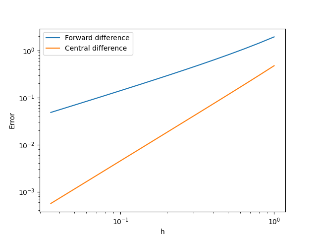
After line 38, the error of the difference approximation calculated above is plotted as a function of the step width (\(h\)). Note that a log-log graph is used here.

From the graph, it can be seen that the error of the forward difference approximation (blue line) and the central difference (orange line) is proportional to different powers of the width \(h\). This behavior is consistent with the error analysis using Taylor expansion discussed above.

Lesson 1-3: Numerical Differentiation of Second Derivatives

In the previous section, we numerically evaluated first derivatives using difference approximations. In this section, we will apply the knowledge gained from the numerical calculation of first derivatives to learn how to numerically evaluate second derivatives.

Consider the following Taylor expansions: \[ f(x+h)=f(x)+f'(x)h+\frac{1}{2}f''(x)h^2+\frac{1}{6}f^{(3)}(x)h^3 + \mathcal{O}(h^4),\] \[ f(x-h)=f(x)-f'(x)h+\frac{1}{2}f''(x)h^2-\frac{1}{6}f^{(3)}(x)h^3 + \mathcal{O}(h^4).\] By subtracting \(2f(x)\) from the sum of these two Taylor expansions, we can create the following difference approximation formula for the second derivative: \[ \frac{f(x+h)-2f(x)+f(x-h)}{h^2}=\frac{d^2f(x)}{dx^2}+\mathcal{O}(h^2). \] Furthermore, the order of error in this difference formula is \(\mathcal{O}(h^2)\).

The following Python code shows a program that numerically calculates the second derivative \(f''(x)\) of the function \(f(x)=\cos(x)\). To get familiar with second derivatives and Python programming, try writing similar code on your own.

(lesson1_3.py)

 from matplotlib import pyplot
 import numpy as np
 
 def second_order_derivative_cos(x,h):
     fx = np.cos(x)
     fx_ph = np.cos(x+h)
     fx_mh = np.cos(x-h)
     d2fdx2 = (fx_ph -2*fx +fx_mh)/h**2
     return d2fdx2
 
     
 h = 0.1
 nx = 52
 xini = 0.0
 xfin = 7.0
 
 x = np.linspace(xini, xfin, nx)
 fx = np.cos(x)
 
     
 d2fdx2 = second_order_derivative_cos(x,h)
 
 
 pyplot.plot(x, fx, label="f(x)=cos(x)")
 pyplot.plot(x, d2fdx2, label="f''(x)")
 
 pyplot.xlabel('x')
 pyplot.ylabel('f(x)')
 pyplot.legend()
 pyplot.savefig("second_derivative_cos.png")
 pyplot.show()

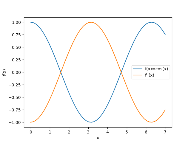
The figure below illustrates \( f(x)=\cos(x) \) and \(f''(x) \) by executing the sample code mentioned above.