Lesson 3: Solving First-Order Differential Equations

Lesson 3-1: Euler's Method

First, we will learn about the most basic numerical solution method for differential equations, known as Euler's method. To introduce Euler's method, let's review the concept of differentiation of a function, similar to the discussion on the forward difference formula in Section 1: Numerical Differentiation. The derivative of a function \(f(x)\) is defined as follows. \begin{align} y'(x)=\lim_{h\rightarrow 0} \frac{y(x+h)-y(x)}{h}. \tag{2} \end{align} Assuming \(h\) is sufficiently small in this equation, the derivative can be approximated using the forward difference formula as follows. \begin{align} y'(x)\approx \frac{y(x+h)-y(x)}{h}. \tag{3} \end{align} Rewriting this equation, we further obtain \begin{align} y(x+h)\approx y(x) + y'(x)h. \tag{4} \end{align}

Looking at equation (4), the right side is written only with the information of \(y(x)\) and \(y'(x)\) at \(x\), and with this information alone, we can approximately evaluate the value of the function at \(x+h\), \(y(x+h)\). Therefore, by sequentially repeating such operations, it is possible to evaluate the value of the function \(y(x)\) at any variable \(x\). This type of numerical solution method for differential equations is called Euler's method. The following figure schematically shows the procedure of the Euler method.

Below, we will explain the procedure of Euler's method in more detail.

1. First, set the initial condition of the differential equation (1), \(y(x_0)=y_0\).
2. Next, by evaluating the function \(f(x_0,y(x_0))\), obtain the derivative value \(y'(x_0)\).
3. Using the evaluated derivative value \(y'(x_0)\), evaluate the function value at \(x_0+h\), \(y(x_0+h)\), through equation (4).
4. Based on the evaluated \(y(x_0+h)\), calculate the function value \(f(x_0+h,y(x_0+h))\) and evaluate the derivative value \(y'(x_0+h)\) at \(x_0+h\).
5. Using the evaluated derivative value \(y'(x_0+h)\), evaluate the function value at \(x_0+2h\), \(y(x_0+2h)\), through equation (4).
6. Repeat the same steps below.

By following these steps, it is possible to numerically solve the differential equation. As an exercise in the numerical solution of differential equations using Euler's method, let's numerically solve the following differential equation under the initial condition \(y(x=0)=1\): \begin{align} y'(x)=-2x y(x). \tag{5} \end{align} Note that the solution to this differential equation is a Gaussian function, \(y(x)=e^{-x^2}\).

Below is an example Python code to solve the above differential equation (5). Use this code as a reference to create your own code for numerically solving differential equations and explore how the accuracy of the solution changes with different step sizes \(h\).

(lesson3_1.py)

 from matplotlib import pyplot as plt
 import numpy as np
 
 # define the derivative, dy/dx
 def dydx(x,y):
     return -2.0*x*y
 
 # Euler method: compute y(x+h)
 def euler_method(y,x,h):
     return y+dydx(x,y)*h
 
 
 # Solve the differential equation from x=a to x=b with n discretized points
 
 a = 0.0
 b = 2.5
 n = 8
     
 h = (b-a)/n
 x_values = np.linspace(a, b, n+1)
 y_values = np.zeros(n+1)
 
 # initial condition, y(a)=y_0
 y_values[0] = 1.0
 
 for i in range(n):
     y_values[i+1] = euler_method(y_values[i],x_values[i],h)
 
 
 # Plot the results
 plt.plot(x_values, y_values, label="Euler method")
 plt.plot(x_values, np.exp(-x_values**2), label="Exact solution", linestyle='dashed')
 
 plt.xlabel('x')
 plt.ylabel('f(x)')
 plt.legend()
 plt.savefig("result_Euler.png")
 plt.show()

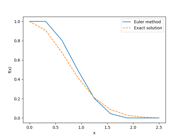
The figure below shows the results obtained by the above source code. In this calculation, the width \(h\) is set to 2.5/8=0.3125. With this step size, Euler's method does not provide an accurate solution and it can be seen that there is a significant error from the exact solution.

Lesson 3-2: Predictor-Corrector Method

In the previous section, we discussed Euler's method as the simplest way to solve differential equations. However, Euler's method is not very accurate and is seldom used in actual computational science applications. In this section, we will explain a more accurate solution method called the Predictor-Corrector Method.

Euler's method was based on the forward difference approximation of equation (3). Here, we consider a more accurate difference formula, the central difference approximation, as follows. \begin{align} \frac{dy\left ( x+\frac{h}{2} \right )}{dx}\approx \frac{y(x+h)-y(x)}{h} \tag{6} \end{align} Furthermore, similar to the case with Euler's method, we make the following rewrite. \begin{align} y(x+h)\approx y(x)+\frac{dy\left ( x+\frac{h}{2} \right )}{dx}h. \tag{7} \end{align}

Here, if we consider approximating the derivative value \( \frac{dy(x+h/2)}{dx} \) at \(x+h/2\) with the average of the derivative values at \(x+h\) and \(x\), we get the following approximation. \begin{align} y(x+h)\approx y(x)+h\frac{f\big ( x+h,y(x+h) \big) + f\big ( x,y(x) \big) }{2}. \tag{8} \end{align}

This formula (8) is a more accurate approximation than Euler's method, but calculating the right side of equation (8) requires the information of the function value \(y(x+h)\) at \(x+h\), making it difficult to use directly in actual calculations. To practically evaluate the value of \(y(x+h)\) on the right side of equation (8), the following two-step process is used.

First, in the initial step of the procedure (predictor step), the approximate value of \(y(x+h)\) at \(x+h\) is evaluated using Euler's method as follows: \begin{align} \bar y (x+h)=y(x)+hf \left (x,y(x)\right). \tag{9} \end{align} Here, the approximate value is denoted by \(\bar y(x+h) \).

In the second step (corrector step), the approximate value \(\bar y(x+h)\) obtained in the previous step is used to evaluate the right side of equation (7), obtaining \(y(x+h)\) as follows. \begin{align} y(x+h) = y(x)+h\frac{f\left ( x+h,\bar y(x+h) \right) + f\left ( x,y(x) \right) }{2}. \tag{10} \end{align}

The numerical method of solving differential equations using the above two-step process is called the Predictor-Corrector method. To compare the accuracy of Euler's method and the Predictor-Corrector method, let's solve the differential equation (5) using the Predictor-Corrector method and compare the results.

Below is a sample Python code to solve the differential equation (5) using the Predictor-Corrector method.

(lesson3_2.py)

 from matplotlib import pyplot as plt
 import numpy as np
 
 # define the derivative, dy/dx
 def dydx(x,y):
     return -2.0*x*y
 
 # Predictor-corrector method: compute y(x+h)
 def pred_corr_method(y,x,h):
     y_bar = y+dydx(x,y)*h
     return y+0.5*h*(dydx(x,y)+dydx(x+h,y_bar))
 
 
 # Solve the differential equation from x=a to x=b with n discretized points
 
 a = 0.0
 b = 2.5
 n = 8
     
 h = (b-a)/n
 x_values = np.linspace(a, b, n+1)
 y_values = np.zeros(n+1)
 
 # initial condition, y(a)=y_0
 y_values[0] = 1.0
 
 for i in range(n):
     y_values[i+1] = pred_corr_method(y_values[i],x_values[i],h)
 
 
 # Plot the results
 plt.plot(x_values, y_values, label="Predictor-corrector method")
 plt.plot(x_values, np.exp(-x_values**2), label="Exact solution", linestyle='dashed')
 
 plt.xlabel('x')
 plt.ylabel('f(x)')
 plt.legend()
 plt.savefig("result_PredCorr.png")
 plt.show()

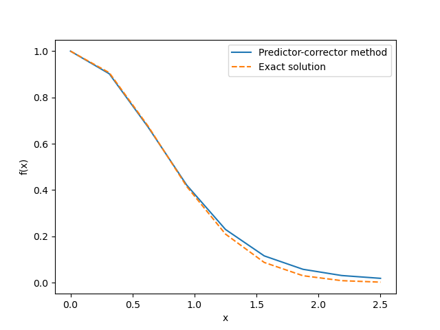
The figure below shows the results obtained by the source code of the Predictor-Corrector method mentioned above. In this calculation, the width \(h\) is set to 2.5/8=0.3125.