Lesson 5: The Monte Carlo Method

Lesson 5-1: An Example of the Monte Carlo Method (Calculating Pi)

In this section, we will learn about the Monte Carlo method. The Monte Carlo method is a numerical computation technique that uses random numbers.

The Python code below is an implementation of the Monte Carlo method for estimating the value of pi (π). This method is based on the principle of statistical probability and uses random numbers to obtain numerical results.

(lesson5_1.py)

 import matplotlib.pyplot as plt
 import random
 
 # Number of random points to generate
 n = 10000
 
 # Initializing counters for points inside and outside the circle
 num_inside_circle = 0
 num_outside_circle = 0
 
 # Lists for storing points for plotting
 x_inside = []
 y_inside = []
 x_outside = []
 y_outside = []
 
 # Generating random points and calculating Pi
 for _ in range(n):
     x, y = random.random(), random.random()
     distance = x**2 + y**2
 
     if distance <= 1:
         num_inside_circle += 1
         x_inside.append(x)
         y_inside.append(y)
     else:
         num_outside_circle += 1
         x_outside.append(x)
         y_outside.append(y)
 
 # Estimating Pi
 pi_estimate = 4 * num_inside_circle / n
 
 # Plotting the points
 plt.figure(figsize=(6,6))
 plt.scatter(x_inside, y_inside, color='blue', s=1)
 plt.scatter(x_outside, y_outside, color='red', s=1)
 plt.title(f'Estimation of Pi using Monte Carlo Method: {pi_estimate}')
 plt.xlabel('X-axis')
 plt.ylabel('Y-axis')
 plt.savefig('pi_mc.png')
 plt.show()

Below is an explanation of the code:

1. Importing Libraries

1. matplotlib.pyplot: Used for plotting the results.
2. random: Used to generate random numbers.

2. Initialization

1. n = 10000: Defines the number of random points to be generated.
2. num_inside_circle and outside_circle: Counter variables to count the number of points inside and outside the unit circle, respectively.
3. x_inside, y_inside, x_outside, y_outside: Lists to store the coordinates of the points for plotting.

3. Generating Random Points and Estimating Pi

1. A loop that runs n times to generate random points.
2. In each iteration, a point (x, y) is generated with random numbers for x and y between 0 and 1.
3. The distance from the origin (0,0) to the point is calculated using the formula \( \text{distance} = x^2 + y^2 \).
4. If the distance is less than or equal to 1, then the point lies inside the unit circle, and the inside_circle counter is incremented. The coordinates of the point are also added to the x_inside and y_inside lists.
5. If the distance is greater than 1, then the point falls outside the unit circle, and the outside_circle counter is incremented. The coordinates of the point are added to the x_outside and y_outside lists.

4. Estimating Pi

1. The estimate of pi is calculated using the formula \( \pi_{\text{estimate}} = 4 \times \frac{\text{inside_circle}}{n} \).
2. This formula is derived from the ratio of the area of the circle to the area of the square. Since the side of the square is 1 (the radius of the circle), the area of the square is 1, and the area of the circle is π/4. Thus, the ratio of points inside the circle to the total number of points approximates π/4.

5. Plotting the Points

1. A scatter plot is created using Matplotlib.
2. Points inside the circle are plotted in blue, and points outside the circle are plotted in red.
3. The plot is titled with the estimate of pi and labeled on the X and Y axes.

6. Displaying the Estimate of Pi

1. Finally, the estimate of pi is displayed.

This method is a probabilistic approach, and the accuracy of the estimate improves with an increased number of generated random points. The plot visually demonstrates how random sampling covers the area of the unit square and the unit circle, explaining the concept behind Monte Carlo estimation.

The above Python code estimates the value of pi using the Monte Carlo method by generating random points and checking whether they fall inside or outside the unit circle. In this simulation, 10,000 points were generated.

The figure below visually represents the distribution of these points, where points inside the circle are shown in blue and points outside the circle are shown in red. This approach approximates the value of pi by utilizing the ratio of the area of the circle to the area of the square. The accuracy of this estimate improves as the number of points used in the simulation increases.

Lesson 5-2: The Monte Carlo Method for Integration

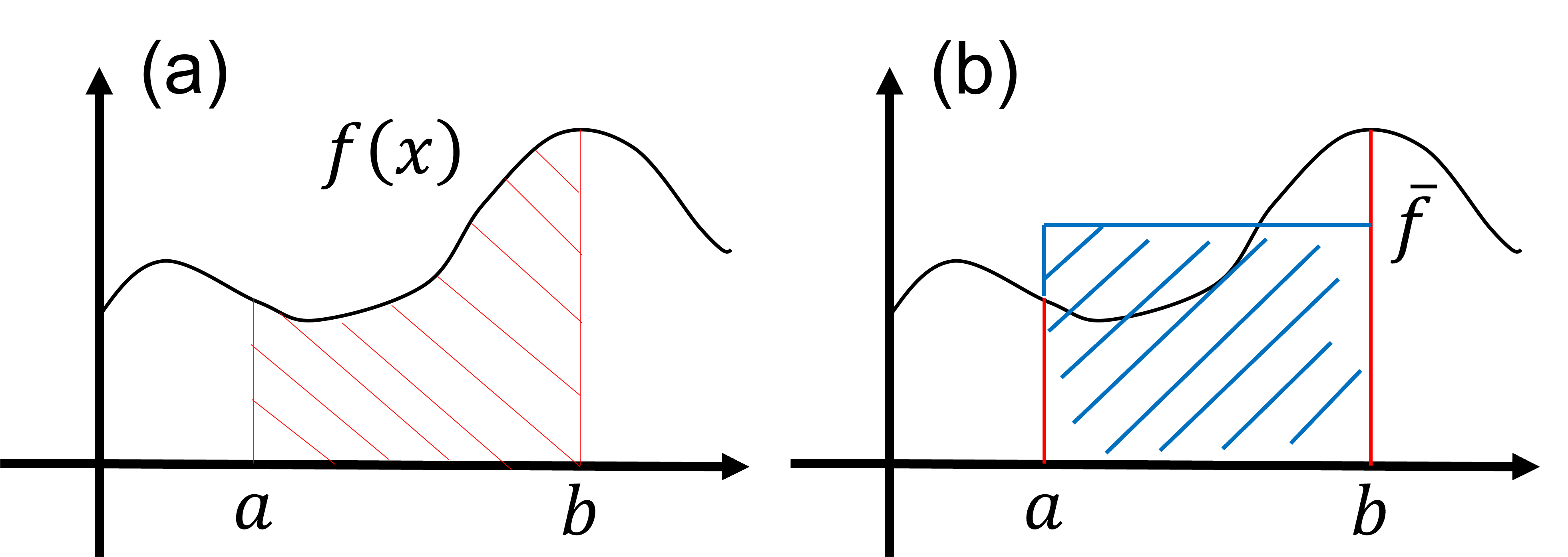
Here, we will learn how to use the Monte Carlo method to integrate a function. Consider the following integral: \begin{align} S=\int^b_a dx f(x). \tag{1} \end{align} The value of the integral \(S\) corresponds to the area painted in red in figure (a) below. It is important to note that the value of the integral also corresponds to the area painted in blue in figure (b). This is described by \begin{align} S=\int^b_a dx f(x)= (b-a)\times \bar f, \tag{2} \end{align} where \(\bar f \) is the average value of the function \(f(x)\) over the range \((a\le x \le b)\). From this observation, it is suggested that the value of the integral \(S\) can be evaluated using the average value \(\bar f \) of the function \( f(x) \) within the range of integration.

The Monte Carlo method for integration is based on evaluating the average value \( \bar f \). In the most basic algorithm of the Monte Carlo method for evaluating the integral (equation \(1\)), many random numbers \(x_i\) are generated within the range \((a \le x \le b) \). The average value \( \bar f \) is then approximated as follows: \begin{align} \bar f \approx \frac{1}{N} \sum^N_{i=1}f(x_i), \tag{3} \end{align} where \(N\) is the number of generated random numbers. Thus, the integral in equation \((1)\) is approximated as follows: \begin{align} S=\int^b_a dx f(x)= (b-a)\times \bar f \approx \frac{b-a}{N}\sum^N_{i=1}f(x_i) \tag{4} \end{align} using the random numbers \(\{x_i \}\) generated within the range \((a\le x \le b)\).

To get accustomed to the Monte Carlo method, let's write a Python program to evaluate the following integral: \begin{align} S=\int^1_0 dx \frac{4}{1+x^2}. \tag{5} \end{align} Integrating equation \( (5)\) analytically, we can obtain \(S=\pi\).

The Python code below is an implementation of the Monte Carlo method to estimate the value of \(S\) for equation \((5)\).

(lesson5_2.py)

import random

# Number of random points to use for the Monte Carlo simulation
n = 10000

# Function to integrate
def f(x):
    return 4.0/(1.0 + x**2)

# Monte Carlo integration
integral = 0.0

for _ in range(n):
    integral = integral + f(random.random())

integral = integral / n

print('integral =',integral)

The Python code above is an example of using the Monte Carlo method for numerical integration. Below is a detailed breakdown of its components and functionality:

1. Importing the Random Module: The code imports the random module, which is used to generate random numbers.
2. Setting the Number of Random Points (n): The variable n is set to 10,000, representing the number of random points used in the simulation. Generally, the greater the number, the more accurate the approximation will be.
3. Defining the Function to Integrate (f(x)): The function f(x) is defined as 4.0 / (1.0 + x**2). This function is part of the equation used to calculate the numerical value of π.
4. Monte Carlo Integration:
   • The variable integral is initialized to 0.0 and accumulates the sum of function values.
   • A for loop runs n times, and each time:
     • A random number between 0 and 1 is generated using random.random().
     • The result of f(x) at this random number is added to integral.
   • After the loop, integral holds the sum of f(x) for all random points.
5. Calculating the Approximate Integral: The sum in integral is divided by n and used to obtain the average value that approximates the integral over the range [0, 1].
6. Printing the Result: The calculated approximate integral is printed.

In summary, this code is an implementation of the Monte Carlo method for estimating the integral of a function over a specific interval. In this case, it is a method for estimating the value of π by approximating the integral of 4/(1 + x^2) over the range [0, 1]. The accuracy of this approximation depends on the number of random points used.

Lesson 5-3: The Monte Carlo Method with General Distributions

In the previous section, we learned about the Monte Carlo method using random numbers from a uniform distribution. In this section, we explore how to apply the Monte Carlo method using general distributions instead of the uniform distribution. Consider the following integral: \[ S = \int^{\infty}_{-\infty}dx f(x) w(x), \tag{6} \] where \( w(x) \) is a non-negative distribution function (i.e., for any \( x \), \( w(x) \ge 0 \)) and is normalized (\( \int^{\infty}_{-\infty} dx w(x) = 1 \)). As long as the distribution function \( w(x) \) satisfies the conditions of non-negativity and normalization, the integral in equation (6) can be evaluated using random numbers distributed according to \( w(x) \), as indicated by the sum below: \[ S = \int^{\infty}_{-\infty}dx f(x) w(x) \approx \frac{1}{N}\sum^{N}_{i=1} f(x_i), \tag{7} \] where \( N \) is the number of random numbers, and \( \{x_i\} \) are random numbers generated according to the probability distribution function \( w(x) \).

Python's random module offers support for generating random numbers from various distributions, including uniform, exponential, and normal distributions. Additionally, random numbers from any distribution can also be generated using Metropolis sampling.

Here, we provide an example of using the Monte Carlo method with general distributions. We consider calculating the following integral using a normal distribution:

\[ S=\int^{\infty}_{-\infty}dx x^2 \frac{1}{\sqrt{2\pi}} e^{-\frac{x^2}{2}}=1. \tag{7} \]

The Python code below is an implementation of the Monte Carlo method to estimate the value of \( S \) for equation (7). (Python code is provided here)

(lesson5_3.py)

import numpy as np

# Number of random points to use for the Monte Carlo simulation
n = 10000

# Function to integrate
def f(x):
    return x**2

# Monte Carlo integration
integral = 0.0

for _ in range(n):
    integral = integral + f(np.random.normal(0, 1))

integral = integral / n

print('integral =',integral)

Lesson 5-4: Importance Sampling

In this section, we will learn about a technique to improve the convergence of Monte Carlo sampling by using appropriate distribution functions corresponding to the integral function. Consider modifying the integral as follows:

\begin{align} S=\int^{\infty}_{-\infty}dx f(x) =\int^{\infty}_{-\infty}dx \frac{f(x)}{w(x)}w(x), \tag{8} \end{align}

Here, \( w(x) \) is a distribution function that satisfies the normalization condition \(\int^{\infty}_{-\infty}dx w(x)= 1\) and guarantees positive values \( w(x) > 0 \). Utilizing the concept from Lesson 5-3, the integral in equation (8) can be evaluated using Monte Carlo sampling. This is done by sampling random numbers according to the distribution function \( w(x) \), as shown in the approximation below:

\begin{align} S = \int^{\infty}_{-\infty}dx \frac{f(x)}{w(x)}w(x) \approx \frac{1}{N}\sum^N_i \frac{f(x_i)}{w(x_i)}, \tag{9} \end{align} where \( N \) represents the number of random numbers used, and \( \{x_i\} \) are random numbers sampled from \( w(x) \).

The convergence rate of Monte Carlo sampling shown in equation (9) is influenced by the variability of the ratio \(\frac{f(x_i)}{w(x_i)}\). Consider a scenario where this ratio is a constant independent of \(x\). In such a case, convergence results can be obtained even with a single Monte Carlo sample. To achieve faster convergence in typical scenarios, it is beneficial to choose a distribution function \(w(x)\) that closely resembles \(f(x)\). This similarity minimizes the variability of the sampled values \(\frac{f(x_i)}{w(x_i)}\) and leads to quicker convergence. Essentially, when the distribution function \(w(x)\) increases in areas where the integral function \(f(x)\) is large, Monte Carlo sampling converges more rapidly. This approach of selecting an optimal distribution function to improve sampling efficiency is known as importance sampling.